3  Selective Logging Detection with Deep Learning and Very-High Resolution Imagery

Authors

Affiliation

Osmar Yupanqui

Conservación Amazónica - ACCA

Marvin Quispe

Conservación Amazónica - ACCA

How to cite this chapter:

Yupanqui, O., & Quispe, M. (2026). Selective Logging Detection with Deep Learning and Very-High Resolution Imagery. Zenodo. https://doi.org/10.5281/zenodo.20547803

Part of: Mayer, T., Bhandari, B., & Saah, D. (2026). EarthRISE Applied Artificial Intelligence and Deep Learning Book. Zenodo. https://doi.org/10.5281/zenodo.20547797

Run in Colab View on GitHub

3.1 Understanding the selective logging activity

Forest conservation faces a threat that is difficult to detect but highly devastating: selective logging. Unlike deforestation, which can be identified relatively easily from space using freely available satellite imagery, selective logging involves the removal of only commercially valuable trees from the forest cover, leaving a deceptive appearance of normality in the forest. For this reason, detecting this activity poses a considerable technological and logistical challenge.

First, the areas of forest loss caused by this activity are typically not detected using medium-resolution remote sensing imagery such as Sentinel-2 and Landsat. This is because tree removal in the forest leaves a small area of ​​impact. Furthermore, the impact is difficult to observe because it occurs below the forest canopy.

Second, there is only a short window after harvesting to assess this activity (2-3 months). This is because tropical forests, especially those in the Amazon rainforest, exhibit high rates of natural regeneration during vegetation succession processes. As a result, signs of disturbance can disappear quickly. Furthermore, the frequency of satellite image acquisition is not always sufficient to detect the activity in time, before it spreads to more remote areas.

Third, the heavy cloud cover in the Amazon region. Cloud cover limits the observation of land cover using optical sensors. In addition, in recent years there has been an increase in cloud cover in some areas of the Amazon; however, the causes of this phenomenon have not yet been thoroughly analyzed.

For this reason, researchers and organizations in the region, such as Conservación Amazónica - ACCA, use commercial satellite imagery from SkySat (0.5-meter spatial resolution), operated by Planet Labs, to monitor selective logging. These images can be acquired on demand and are updated daily, making them a particularly well-suited tool for monitoring remote areas.

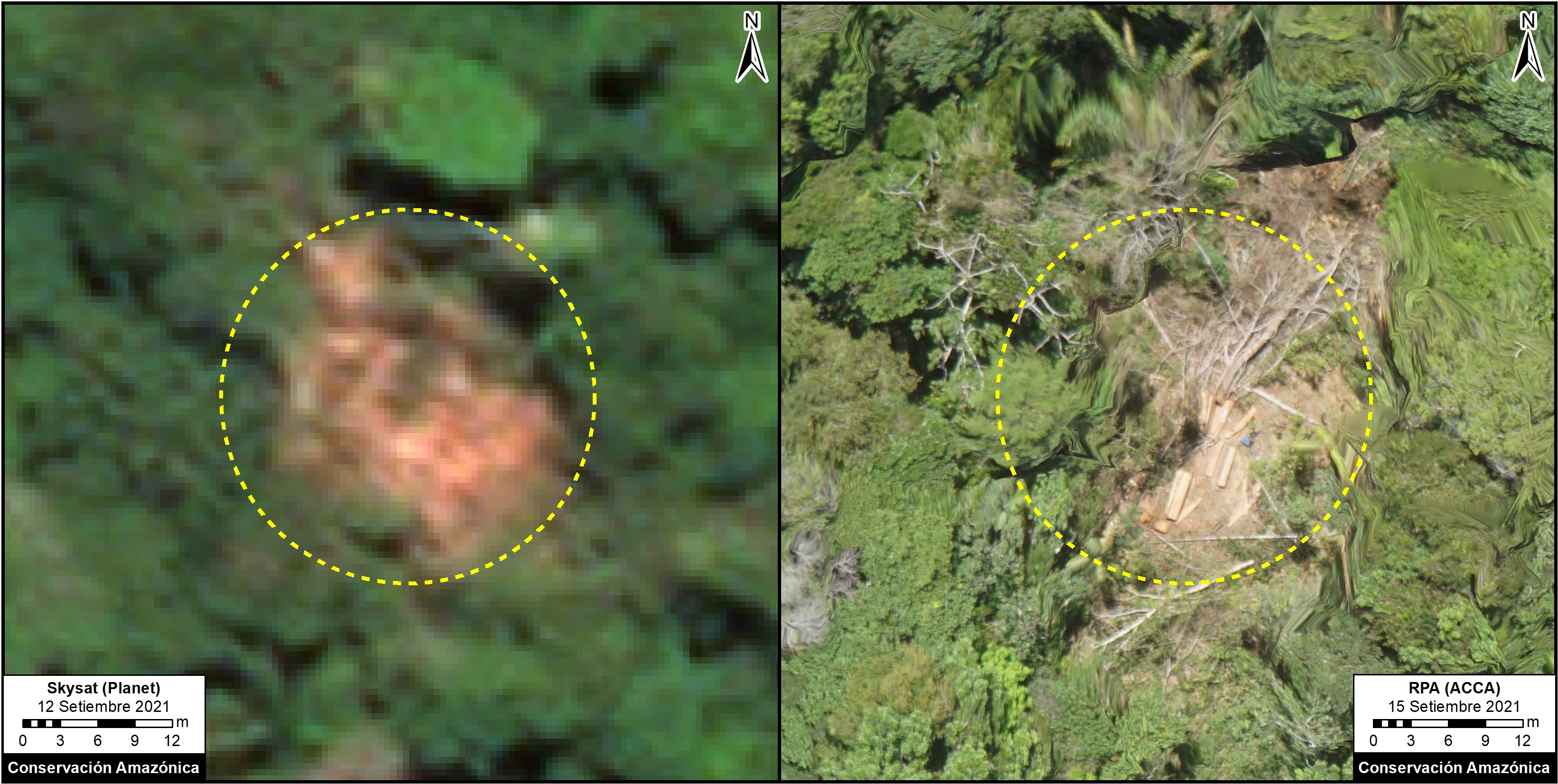
Below is an image comparing, in the same location, logging activity with a SkySat image (0.5 m) and a drone image (3 cm). Logs are visible, and a blue canister can be seen for refilling fuel for the chainsaws used for logging.

Comparison between a SkySat image (0.5 m) and a drone image (3 cm)

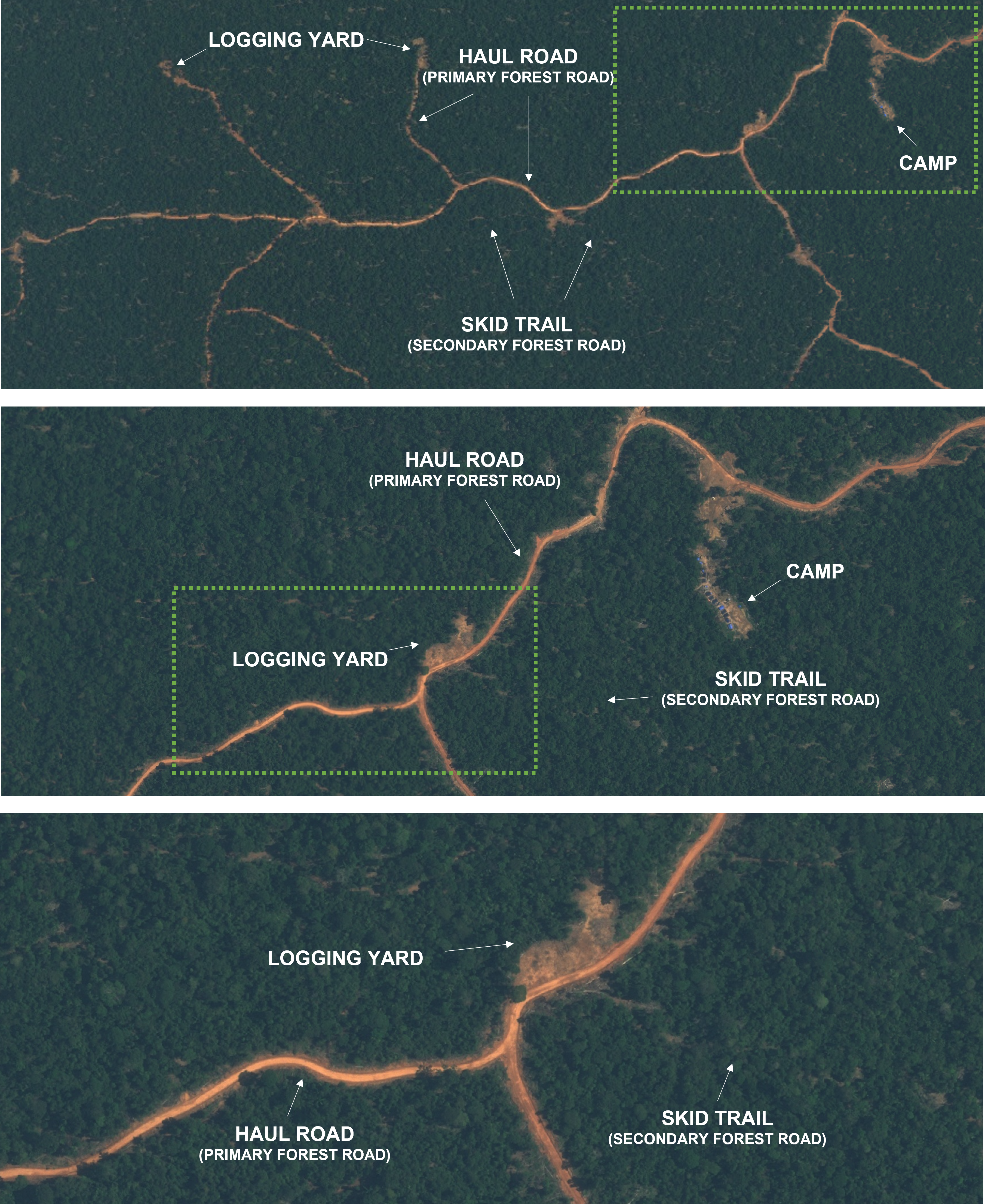
Selective logging is often associated to infrastructures such as logging roads, logging yards, camps, among others. Identifying these critical infrastructures makes it easier to detect logging activities. The presence of these infrastructures occurs in areas where logging is common, such as timber forest concessions and forest plantations. However, in remote areas where the activity is generally illegal, it is possible to observe a network of trails, usually beneath the forest canopy.

Diferent infrastructures associated with selective logging

3.2 Part I: Data processing and exporting

Due to the growing volume of available satellite data and the need for researchers and organizations to process it efficiently, cloud platforms such as Google Earth Engine (GEE). have become widely used tools in geospatial analysis. GEE allows users to access and process large collections of satellite data without needing to download them locally, which significantly reduces computational requirements; for this reason, it is currently one of the most used platforms for geospatial analysis. Additionally, it offers a free plan, as well as commercial options for users with greater processing and storage needs.

This section presents a simple workflow for processing satellite data on the Google Earth Engine (GEE) platform and exporting it to an optimized format (TFRecord) to Google Drive. It should be noted that all sections in this application example have been developed to run on Google Colab (free version), using CPUs for reference data export and inference (Part I and Part III), and GPUs for model training (Part II). Therefore, we recommend using this platform for execution. If you wish to run it locally, we suggest using Visual Studio Code, after installing the Google Colab VS Code Extension.

All the files needed to implement this application example are available on GitHub. In addition, the benchmark data used can be found on Zenodo. We recommend downloading and reviewing its contents to better understand the data structure or, if you prefer, proceeding directly to model training (Part II). However, it is not necessary to download it to run this section (Part I), as it includes the process of exporting the reference data from scratch directly to Google Drive. The complete export of the reference data takes approximately 1 hour and 20 minutes and generates a set of files with a total size of approximately 17 MB.

To avoid future complications and as a good practice, create the main working folder named DL_Book before running the main code. This folder should be located in the main storage path; in our case, on Google Drive.

# We are going to connect Google Drive with Google Colab
from google.colab import drive
drive.mount('/content/drive')

# Next, we create the main working folder
import os
os.makedirs('/content/drive/MyDrive/DL_Book', exist_ok = True)

Additionally, print the available computational resources in Google Colab to understand the characteristics of the environment in which the notebook will run.

print("─── Google Colab resources report ───")
!echo -n "CPU Model: " && lscpu | grep "Model name" | cut -d':' -f2 | xargs
!echo -n "Total RAM: " && free -h | awk '/Mem:/ {print $2}'
!echo -n "Available Disk: " && df -h / | awk 'NR==2 {print $4 " of " $2}'
!echo -n "GPU: " && (nvidia-smi --query-gpu=name --format=csv,noheader 2>/dev/null || echo "Not available")

3.2.1 Setting up your Google Earth Engine account

The Google Earth Engine Python API requires a personal account. For enabling the API you need the following:

• A Google account linked to Google Earth Engine.
• A Google Cloud Project (A non-commercial project is suggested).

For detailed information on how to create a GEE account and set up a project on Google Cloud (including enabling the API, selecting the non-commercial use option, and reviewing quota levels), we recommend that you refer to the following notebook.

3.2.2 Data exploration

First, we will import the official Earth Engine library in Python, for the data visualization and processing, using import

import ee

Because the Earth Engine API requires a personal account, we will proceed to authenticate our account and initialize Earth Engine. When we run the following cell, a link will appear, where we must provide authorizations. Note that we have to introduce our project ID in ee.Initialize().

ee.Authenticate()
# Replace 'my-project' with your project id
ee.Initialize(project = 'my-project')

Finally, we will import another important library called Geemap, which will allow us to visualize the data using ipyleaflet. If we do not have geemap, we can download it using the !pip install command.

import geemap

Using the Earth Engine API we can visualize the data using python and geemap. We will load a very high resolution (0.5 m) SkySat satellite image as well as the collected training data (polygons).

img = ee.Image('projects/ACCA-SERVIR/Colaboraton/Skysat_Fatima') # This imports the SkySat image as an ee.Image()
polygons = ee.FeatureCollection('projects/ACCA-SERVIR/Colaboraton/Skysat_Fatima_pols') # This imports the data (polygons) that will be further used in the training, as an ee.FeatureCollection()

The Geemap library is very useful for visualizing our data.

Map = geemap.Map(center = (-9.653, -74.198), zoom = 15) # This creates a map using ipyleaflet
Map.addLayer(img, {'bands': ['b3', 'b2', 'b1'], 'min': 2000, 'max': 8000}, 'SkySat') # This adds our image to the map, with custom visualization parameters
Map.addLayer(polygons, {'color': 'red'}, 'Training Polygons') # This adds the imported polygons to the map
Map

We will also print the amount of polygons that we have.

print(polygons.size().getInfo()) # The .size() method retrieves the amount of polygons in our feature collection, .getInfo() brings the response to the client synchronously

3.2.3 Data processing

3.2.3.1 Assign a numerical value to the class

This workflow is designed for a binary semantic segmentation, for this, we need an image label, that matches the projection and size of our input image. This image label will require two values:

• Value of 1: this is what we want to detect (logging).
• Value of 0: the background (forest, water, etc.).

Our database consists of polygons, which all have a string attribute called tipo (type in english), which is not numeric. We will create a function to create an attribute called class with the value of 1 in our feature collection. If this exercise were a multiclass segmentation, more types besides tala (logging) would be expected.

We will print the attributes of the first polygon. Note that it is advisable to have attributes that refer to the image used in the digitalization of the polygons.

Notice the attributes at the end.

print(polygons.first().getInfo())

This creates the function to create an attribute called class with the value of 1. Since all of our polygons are logging, a filter won’t be needed.

def add1(f):
    return f.set('class', 1.0) # The .set() method creates an attribute in each feature

We will print the first feature in our collection, notice the presence of the new attribute created.

polygons = polygons.map(add1) # With the .map() method we apply a function to each feature inside of our feature collection
print(polygons.first().getInfo())

3.2.3.2 Create the “class” band of the image

As we mentioned before, we need an image label. For this, we will create a band, using our processed polygons. This image label will have two pixel values, 1 for logging and 0 for everything else (background).

To do this, we will create a function that transforms our feature collection (polygons) to a binary image.

def createLabel (feature):
    featImg = feature.reduceToImage(['class'], ee.Reducer.mean()) # The .reduceToImage() method transforms our polygons to an image, with a mean reducer
    return featImg.toByte().rename('class') # We will return the image with a byte representation, this is memory efficient

Now, we apply the createLabel() function and add the created band to our SkySat image.

img = img.addBands(createLabel(polygons)) # The .addBands() method adds an image (or band) to another image

Again, we print the bands in the image. Note the existence of the band class, which will become the label, in this case logging.

print(img.bandNames().getInfo())

Let’s visualize our newly created label! You will see that it is very similar to the previou ipyleaflet map. But now our label is an image, instead of a feature collection (polygons).

Map = geemap.Map(center = (-9.653, -74.198), zoom = 15) # This creates a map using ipyleaflet
Map.addLayer(img, {'bands': ['b3', 'b2', 'b1'], 'min': 2000, 'max': 8000}, 'SkySat') # This adds our image to the map, with custom visualization parameters
Map.addLayer(img.select('class'), {'min': 0, 'max': 1, 'palette': ['red']}, 'Image label') # This is our target, the image label, selected from the image
Map

3.2.3.3 Image transformation

There are 3 ways of exporting our data:

• Exporting the whole image, then with a GIS Software or with programming, split the whole image into patches of equal size.
• Using the .getPixels() method.
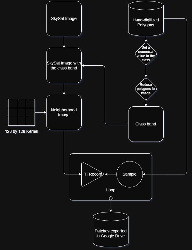
• Transforming our image to a neighborhood image, then exporting individual points (we will use this).

For the third method, we will transform our SkySat image (including the class band). In this neighborhood image, each pixel is a matrix representation of its neighboring pixels. This allows that when exporting a point, the neighborhood its contained as attributes (tensors).

For this, a kernel or matrix is needed. To build a kernel we will use a repetition of lists, with the value of 1 (this value is the weight that each component of the matrix will have).

Note that the size of the kernel will be the size of each exported patch. It is very important that the patch size/kernel contains the object that we want to detect. For this exercise we will export image patches with a size of 128 by 128.

row = ee.List.repeat(1, 128) # This creates a list of 128 numbers with the value of 1
rows = ee.List.repeat(row, 128) # This repeats 128 times the previously creataed list
kernel = ee.Kernel.fixed(128, 128, rows) # This creates our kernel, with a size of 128.

We can print our kernel. Note that it has a size of 128 pixels wide, and 128 pixels height.

print(kernel.getInfo())

Using the kernel, we can perform the image transformation, with the .neightborhoodToArray() method.

img_final = img.neighborhoodToArray(kernel, 0) # The value of 0 adds the background value to the masked pixels

Finally, we will select the predictor variables, which will be part of the export and training.

featureNames = ['b1', 'b2', 'b3', 'b4', 'class']
img_final = img_final.select(featureNames)

To verify, we will print the bands.

print(img_final.bandNames().getInfo())

3.2.4 Data export

In machine learning and deep learning, it is common practice to divide the benchmark dataset into training, validation, and test subsets. The training set is used to adjust the model’s parameters, that is, to enable the algorithm to learn the patterns present in the data. The validation set is used to adjust the hyperparameters and monitor the model’s performance during training, allowing for the detection of issues such as overfitting. Finally, the test set is reserved for conducting a final, independent evaluation of the model, providing an objective estimate of its ability to generalize to unseen data.

The purpose of splitting the benchmark data is to ensure adequate model performance and to objectively evaluate that performance during the training process; therefore, this split is essential and is guided by various strategies and methodological criteria.

For example, a widely used ratio in machine learning, due to its alignment with the Pareto principle, is the 80:20 split between training and testing. From this basic configuration, multiple variations have emerged, most of which now incorporate a validation set. These ratios depend, to a large extent, on factors such as the amount of available data, the heterogeneity of the information, and the complexity of the problem being modeled. Consequently, it is possible to adjust the proportion of data allocated to training by reducing or expanding the validation and test sets according to the specific needs of the analysis, but, generally, without straying too far from the most common ratios, such as 80:20 (training/testing) or its variant, 70:20:10 (training/validation/testing). An inappropriate data splitting strategy can compromise the proper evaluation of the model and lead to unreliable performance estimates.

In this workflow, the dataset (polygons) will be divided into training (70%), validation (20%), and test (10%) subsets. Similar proportions have been used in other studies; for example, Slagter et al. (2024) used a 75/15/10 (training/validation/testing) split in the monitoring of forest roads in the Republic of the Congo.

First, we will assign a random value to each polygon using the .randomColumn() method. Then, we will sort the dataset based on this random value and split the polygons into training, validation, and test subsets.

# Create random column
pols_final = polygons.randomColumn('random', seed=42)  # This creates a column in our feature collection, each feature will have a random value between 0 and 1.

# Sort polygons by the random value
pols_sorted = pols_final.sort('random')  # Sorting ensures a reproducible and deterministic split

print(pols_sorted.first().getInfo())

We can see that the first polygon now has an additional attribute called random, which is used to reproducibly sort the dataset. Based on this ordered random value, we then split the dataset into training, validation, and test subsets using exact proportions.

# Get total number of polygons
n = pols_sorted.size()

# Compute exact split sizes
n_train = n.multiply(0.7).int()  # 70% for training
n_val = n.multiply(0.2).int()    # 20% for validation
# The remaining polygons will be used for testing

# Convert FeatureCollection to list for slicing
pols_list = pols_sorted.toList(n)

# Create exact partitions
training_pols = ee.FeatureCollection(pols_list.slice(0, n_train))
validation_pols = ee.FeatureCollection(pols_list.slice(n_train, n_train.add(n_val)))
testing_pols = ee.FeatureCollection(pols_list.slice(n_train.add(n_val), n))

We can verify the number of training, validation and test polygons.

print(training_pols.size().getInfo())
print(validation_pols.size().getInfo())
print(testing_pols.size().getInfo())

We will create lists in which the polygons will be included.

trainingList = training_pols.toList(training_pols.size())
validationList = validation_pols.toList(validation_pols.size())
testingList = testing_pols.toList(testing_pols.size())

Finally, the data is exported to Google Drive (it can also be exported to Google Cloud Platform or an asset). A loop will be used to export a random pixel of our processed image, that intersects with the polygons, into a TFRecord file (this is the sampling). Remember that each pixel of the image is a representation of its neighborhood (128 by 128), so we are exporting patches as a TFRecord. We will use the for statement for this.

Notice that we are exporting our data into a Google Drive folder called DL_Book, feel free to change it but remember the path.

for i in range(training_pols.size().getInfo()):
    sample = img_final.sample( # The .sample() method samples a feature inside a region
        region = ee.Feature(trainingList.get(i)).geometry(), # This defines the region, in this case, inside each polygon
        scale = 0.5, # The scale, SkySat have a 0.5 m of spatial resolution
        numPixels = 1, # We will only be exporting 1 pixel/1 patch of 128 by 128 per polygon, you can adjust this value to increase the number of patches per polygon
        seed = i,
        tileScale = 8
    )
    trainingTask = ee.batch.Export.table.toDrive(
        collection = sample, # We will export the sample (an individual point inside each of our polygons)
        description = 'train_' + str(i),
        folder = 'DL_Book', # The Google Drive folder that will contain the patch (Feel free to change it)
        fileNamePrefix = 'train_' + str(i), # The name of the file
        fileFormat = 'TFRecord', # The format, currently only TFRecord and GeoTIFF are supported
        selectors = featureNames # The bands that will be exported
    )
    trainingTask.start()
print('Training Data Exported')

for i in range(validation_pols.size().getInfo()):
    sample = img_final.sample(
        region = ee.Feature(validationList.get(i)).geometry(),
        scale = 0.5,
        numPixels = 1,
        seed = i,
        tileScale = 8
    )
    validationTask = ee.batch.Export.table.toDrive(
        collection = sample,
        description = 'validation_' + str(i),
        folder = 'DL_Book',
        fileNamePrefix = 'validation_' + str(i),
        fileFormat = 'TFRecord',
        selectors = featureNames
    )
    validationTask.start()
print('Validation Data Exported')

for i in range(testing_pols.size().getInfo()):
    sample = img_final.sample(
        region = ee.Feature(testingList.get(i)).geometry(),
        scale = 0.5,
        numPixels = 1,
        seed = i,
        tileScale = 8
    )
    testingTask = ee.batch.Export.table.toDrive(
        collection = sample,
        description = 'testing_' + str(i),
        folder = 'DL_Book',
        fileNamePrefix = 'testing_' + str(i),
        fileFormat = 'TFRecord',
        selectors = featureNames
    )
    testingTask.start()
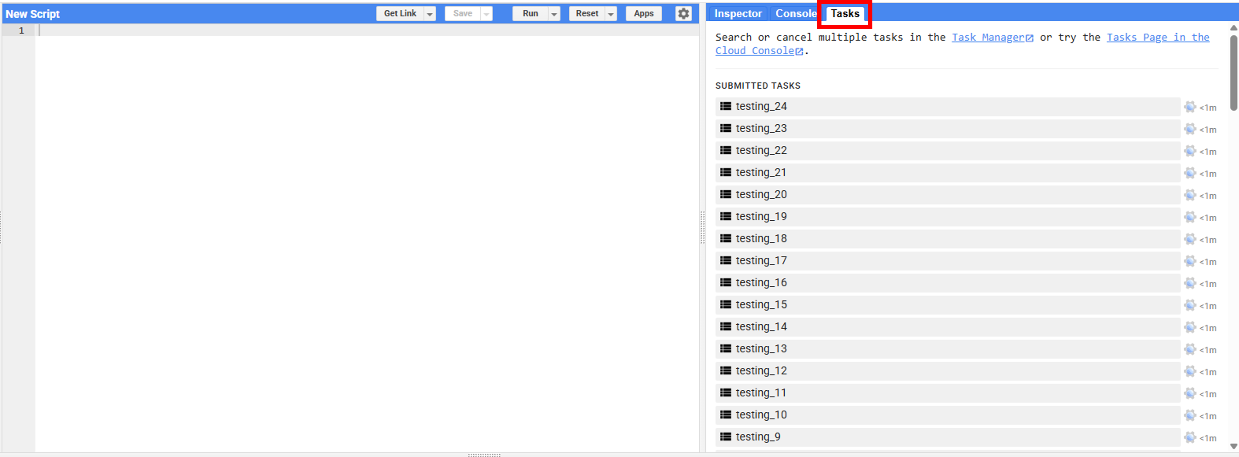
print('Test Data Exported')

You can check the status of your exports in the Google Earth Engine Code Editor, specifically in the Tasks tab. There, you can view the status of each of your tasks. It’s important to monitor them to identify potential export errors or check their progress.

GEE Tasks (Code Editor)

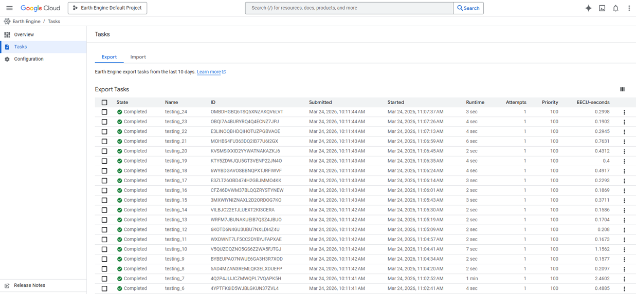
Additionally, there are options for monitoring task status in a more advanced way. Currently, it has also become important to evaluate the quota consumption (EECU) associated with exports. For this type of more detailed analysis, we recommend using the Google Cloud Platform, accessing the Tasks section and supplementing it with “Monitoring Tool” to explore metrics and platform resource usage.

GEE Tasks (GCP)

The workflow summarizes the steps followed in this section.

Data processing and exporting workflow

3.3 Part II: Modeling

This section shows the workflow used to train a deep learning model with the patches saved from the previous section (Part I). We will load our TFRecords, train a model with them and save it for further use (inference). The notebook was developed and configured specifically to run on Google Colab, so its implementation is optimized to run on that platform. In addition, it is necessary to configure the environment to enable GPU computing by changing the runtime type. First, navigate to Edit → Notebook Settings and select GPU from the Hardware Accelerator options.

3.3.1 Data collection and initial settings

We are going to connect Google Drive with Google Colab to manage the exported data (patches) from the previous section.

from google.colab import drive
drive.mount('/content/drive')

If you have not completed Part I, you will need to download the benchmark data, which is stored at: Yupanqui Carrasco, O., & Quispe Sedano, M. J. (2026). Selective Logging Detection with Deep Learning and Very-High Resolution Imagery_TF_records [Data set]. Zenodo. https://doi.org/10.5281/zenodo.19614389

import os
import zipfile
import requests
import io

# Settings
use_drive = True  # True = save to Google Drive, False = save to /content

if use_drive:
    base_path = "/content/drive/MyDrive/DL_Book"
else:
    base_path = "/content/DL_Book"

# Zenodo file URL
url = "https://zenodo.org/api/records/19614389/files-archive"

zip_path = os.path.join(base_path, "dataset.zip")

# Setup directory
os.makedirs(base_path, exist_ok=True)

# Download file
print("Downloading dataset...")
response = requests.get(url, stream=True)

with open(zip_path, "wb") as f:
    for chunk in response.iter_content(chunk_size=8192):
        if chunk:
            f.write(chunk)

print(f"Downloaded to: {zip_path}")

# Extract files
print("Extracting final files...")

with zipfile.ZipFile(zip_path, 'r') as outer_zip:
    for member in outer_zip.infolist():    

        if member.filename.endswith(".zip"):
            print(f"Found inner zip: {member.filename}")
            
            with outer_zip.open(member) as inner_file:
                inner_bytes = io.BytesIO(inner_file.read())
                
                with zipfile.ZipFile(inner_bytes) as inner_zip:
                    for inner_member in inner_zip.infolist():
                        filename = os.path.basename(inner_member.filename)
                        
                        if not filename:
                            continue
                        
                        target_path = os.path.join(base_path, filename)
                        
                        with inner_zip.open(inner_member) as source, open(target_path, "wb") as target:
                            target.write(source.read())

print(f"Final files extracted to: {base_path}")

# Delete zip
os.remove(zip_path)
print("Zip file removed.")

Let’s see the contents of our Drive folder using the linux command !ls.

Note: This command only runs on Google Colab.

!ls -F /content/drive/MyDrive/DL_Book

Our folder should contain several files whose names begin with:

• train.
• testing.
• validation.

Those files are our exported patches from the previous section. If you do not wish to run the previous section , you can create a copy from the original folder. Click here to go to the Drive folder. Make sure to modify the paths to match the current section.

We will also import some libraries that will contribute to the training of the model. This section was built and tested using Google Colab, so the libraries used correspond to the latest version available on this platform at the time of construction and testing (e.g. Tensorflow 2.19.0). Check the latest versions of TensorFlow here.

import tensorflow as tf
print(tf.__version__)

Numpy is another important library, that allow us to perform operations with tensors, matrices and vectors.

import numpy as np

We will also import Matplotlib, for the data visualization.

import matplotlib.pyplot as plt

Finally, we will also import os, to read files and manipulate paths.

import os

3.3.2 Data visualization

First, we will analyze a single TFRecord file, if we explore the folder where the files were downloaded, we can see that they are “compressed” with a special .gz format, Tensorflow allows the use of this special format, without the need to decompress the files.

We will start by creating a variable called record, which will include in a container tf.data.TFRecordDataset() the path of an exported file. Please verify that the export path is the same, in the previous example we exported our data to the DL_Book folder in Google Drive

record = tf.data.TFRecordDataset('/content/drive/MyDrive/DL_Book/testing_0.tfrecord.gz', compression_type = 'GZIP') # This loads our TFRecord into a TFRecordDataset container
print(record)

We can see that the TFRecordDataset does not show all the information, we cannot know the shape of the tensors, even though we know based on the previous code that they have a 128 by 128 shape. We also cannot know the dtype (the data type) neither the number of elements that our TFRecordDataset has.

Because TFRecords are binary storage files, we must transform them into a readable structure. To do this, we will create a dictionary that contains the bands that we exported in the previous code and assign each band a shape with tf.io.FixedLenFeature() and a data type.

features = {
    'b1': tf.io.FixedLenFeature([128, 128], tf.float32),
    'b2': tf.io.FixedLenFeature([128, 128], tf.float32),
    'b3': tf.io.FixedLenFeature([128, 128], tf.float32),
    'b4': tf.io.FixedLenFeature([128, 128], tf.float32),
    'class': tf.io.FixedLenFeature([128, 128], tf.float32),
}

We will create a function to read a serialized example into the structure defined by the dictionary created above.

def parse_tfrecord(example_proto):
    return tf.io.parse_single_example(example_proto, features) # This parses each TFRecord to a defined structure

We will apply the newly created function to our TFRecordDataset using the .map() function, which allows iterating through each element of our TFRecordDataset.

serialized = record.map(parse_tfrecord) # With .map() we loop through each element of our TFRecordDataset
print(serialized)

We can see that the newly created object named serialized has a different form than the original TFRecordDataset. This new object has the structure defined by the dictionary created.

To display the numerical values of each of the bands of our new object, we will use the function get_single_element().

element = serialized.get_single_element() # With .get_single_element() we retrieve an individual element from our TFRecordDataset
print(element)

The result is a dictionary, from which we can extract each band using get() followed by the key, which in this case is the name of the exported band.

b1 = element.get('b1')
b2 = element.get('b2')
b3 = element.get('b3')
b4 = element.get('b4')
label = element.get('class')

We can now view the numerical values ​​of any exported band. We can also transform the objects to a numpy array using the numpy() function.

Now, we will create an “image” to be able to visualize it, concatenating the values ​​of the created bands, into a single tensor.

img = tf.constant([b3.numpy(), b2.numpy(), b1.numpy()]) # This appends each band to a constant tensor
print(img)

If we visualize the shape of the tensor, we see that it has the shape of (3, 128, 128), in order to plot it we must transform the shape to (128, 128, 3). To do this we will use the .transpose() function. In addition, since Matplotlib does only tolerate values from 0 to 255, we will normalize our image (tensor) with .divide().

imgRGB = tf.transpose(tf.divide(img, 12000), [1, 2, 0])

Now, we will plot the results using the matplotlib library. We will be able to contrast how the logging activity is visualized with a SkySat (0.5 m) image (on the left), and the hand-digitized label (on the right).

fig, axs = plt.subplots(1, 2, figsize = (15, 15))

axs[0].set_title('RGB Image')
axs[0].imshow(imgRGB)

axs[1].set_title('Label')
axs[1].imshow(label.numpy())

plt.show()

This plot compares the exported SkySat satellite image patch with the hand-digitized label. Performing the manual digitization process takes many hours, especially when the logging activity is intense. Deep Learning models greatly speed up this manual process and allow the user to focus on evaluating the output.

3.3.3 Data processing

3.3.3.1 Definition of variables

Before performing data processing, some variables will be defined for the training.

• The variable kernel_size contains the size of the patch, from which we build its shape.
• The variable patch_path refers to the folder containing the previously exported patches.
• buffer_size this number is the amount of data that will be filled when shuffling. For example, if our data contains 100 records and we have a buffer_size of 10, then shuffle will select a random element from the first 10 records. The space of this element will be replaced by the 101-st element. Since our dataset contains less than 250 files, and we want the model to shuffle randomly the whole dataset then we will define this parameter to 1000 (it could be higher).

The model also needs hyperparameters, defining these parameters can sometimes be time consuming and experimental. Some of the most important are described below:

• batch_size: The number of examples used in a pass throught the network. A high batch size can lead to faster training times but may result in lower accuracy and overfitting, while a small batch sizes can provide better accuracy, but can be computationally expensive and time-consuming. We will set our batch size to 4 (because this is a small dataset).
• epochs: This is the amount of training cycles through all of the samples in the training dataset. This is how many times the model will see the entire training data before completing training. We will set this value to 10.
• learning_rate: This controls how much the model’s parameters are adjusted during each training step. This will be set to 0.1.

bands = ['b1', 'b2', 'b3', 'b4']
response = ['class']
features = bands + response

kernel_size = 128
kernel_shape = [kernel_size, kernel_size]

columns = [
  tf.io.FixedLenFeature(shape = kernel_shape, dtype = tf.float32) for k in features
]

# Path to the folder with patches (Benchmark dataset)
patch_path = '/content/drive/MyDrive/DL_Book'
train_path = f'{patch_path}/train*'
val_path   = f'{patch_path}/validation*'
test_path  = f'{patch_path}/testing*'

features_dict = dict(zip(features, columns))

train_size = len([f for f in os.listdir(patch_path) if f.startswith('train')])
val_size = len([f for f in os.listdir(patch_path) if f.startswith('validation')])
test_size = len([f for f in os.listdir(patch_path) if f.startswith('testing')])

# Hyperparameters
batch_size = 4
epochs = 10
buffer_size = 1000
learning_rate = 0.1

3.3.3.2 Create a TFRecordDataset

TFRecordDataset are a collection of TFRecords, so they are very useful for storing large amounts of data, and are optimized to save memory.

First, we will create a function called .parse_tfrecord(), which will perform the same functionality as in the data visualization, done previously. We will transform the structure of each TFRecord.

def parse_tfrecord(example_proto):
    return tf.io.parse_single_example(example_proto, features_dict)

Second, a function called .to_tuple() will be created, which will convert the tensor dictionary to a tuple, with the scheme (inputs, outputs).

def to_tuple(inputs):
    inputsList = [inputs.get(key) for key in features]
    stacked = tf.stack(inputsList, axis = 0) # This stacks the input list to a single tensor
    stacked = tf.transpose(stacked, [1, 2, 0]) # Transposition of the stacked tensor to the shape 128x128x4
    return stacked[:, :, :len(bands)], stacked[:, :, len(bands):]

Third, a function will be created to read the tensors, this function will also apply the functions created previously: .parse_tfrecord() and .to_tuple().

def get_dataset(pattern):
    glob = tf.io.gfile.glob(pattern) # This reads the files in our path
    dataset = tf.data.TFRecordDataset(glob, compression_type = 'GZIP') # Add the files to a TFRecordDataset container
    dataset = dataset.map(parse_tfrecord, num_parallel_calls = 5)
    dataset = dataset.map(to_tuple, num_parallel_calls = 5)
    return dataset

We will create 3 TFRecordDataset, which will contain our training, validation and test data set, respectively. To do this we will use functions, within each one there will be an object called glob that will indicate the path of the data sets.

def get_patch_from_path(path, batch_size, buffer_size = 1000, shuffle = False, repeat = False):
    dataset = get_dataset(path + '*')
    dataset = dataset.shuffle(buffer_size, seed = 42) if shuffle else dataset # We will shuffle only the training dataset
    dataset = dataset.batch(batch_size)
    dataset = dataset.repeat() if repeat else dataset
    return dataset

training_data = get_patch_from_path(train_path, batch_size = batch_size, buffer_size = buffer_size, shuffle = True, repeat = True)
validation_data = get_patch_from_path(val_path, batch_size = 1, repeat = True)
testing_data = get_patch_from_path(test_path, batch_size = 1)

If we print the 3 sets of data we will see that the training and validation data we see are of type RepeatDataset(), that is, they are files that are constantly being generated, which based on the previous functions are being ordered randomly and the Outgoing data set has a size of 1 (based on batch size).

print(training_data)
print(validation_data)
print(testing_data)

3.3.4 Deep learning

3.3.4.1 Model construction

In this notebook we will use a modification of the U-Net architecture developed by Ronneberger et al., (2015). The U-Net architecture was initially designed for use in biomedical imaging but proved to be very efficient in the segmentation of satellite and drone images, and is currently one of the most widely used for that purpose. This architecture has demonstrated remarkable effectiveness in various environmental monitoring applications, including agricultural field boundary detection John & Zhang, 2022, urban land use classification, and coastal change detection. Ulmas & Liiv, 2020 further validated U-Net’s superiority in crop type mapping from multi-spectral satellite imagery, showing that its ability to preserve spatial resolution through the decoder path results in more precise segmentation boundaries compared to traditional convolutional neural networks or patch-based classification approaches. The architecture’s robustness to varying image resolutions and its capacity to learn from limited training data through effective data augmentation make it particularly well-suited for remote sensing applications where high-quality labeled data may be scarce Manos et al., 2022.

To represent the architecture we will use some layers of tensorflow.keras. This modified version of U-Net has more encoding and decoding blocks than the original architecture, which increases the depth of the model and its learnability. Unlike the original design, which starts and ends with 64 filters, this implementation starts and ends with a layer of 32 filters, slightly reducing the initial complexity before continuing with the standard progression. Below is a diagram of the modified U-Net architecture used.

Modified U-Net architecture

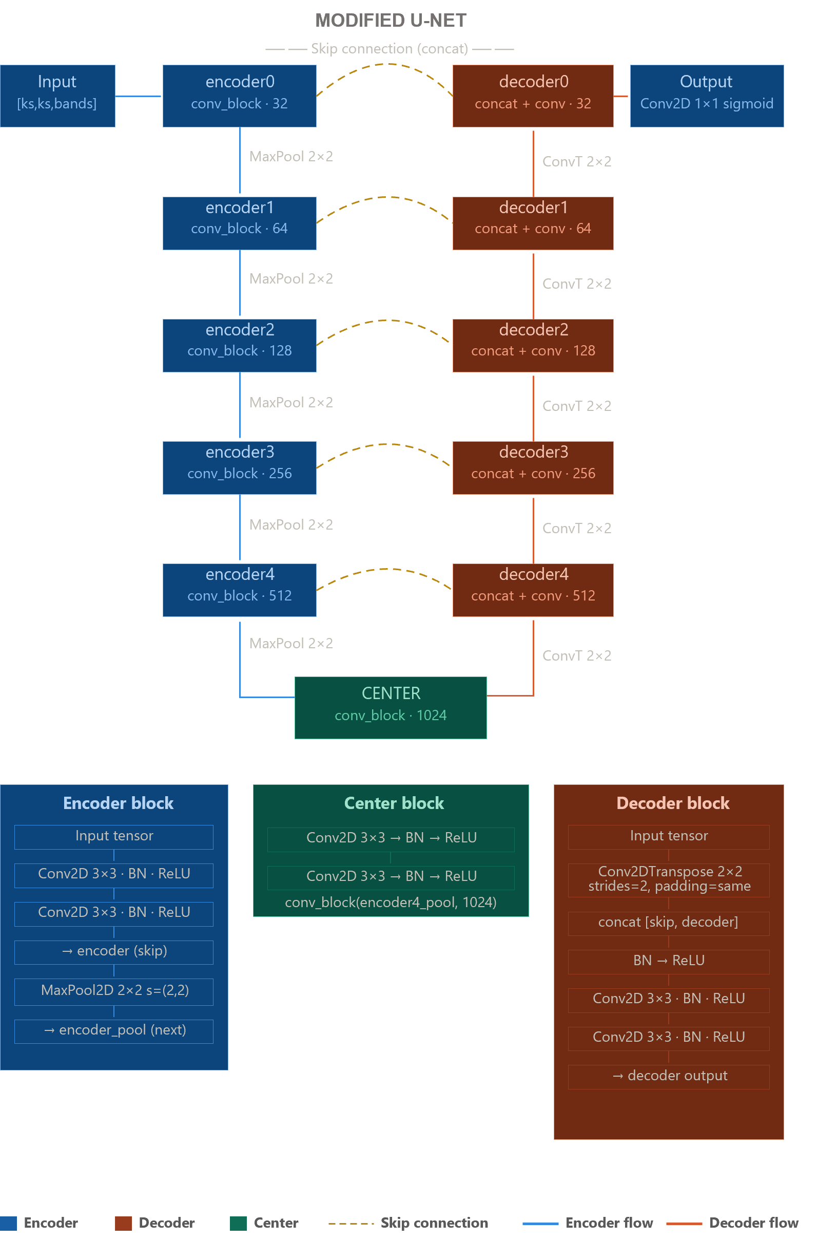
This modified architecture allows a superior multi-scale feature extraction (due to the additional encoder and decoder levels). However, this comes with a cost, this architecture has much more parameters compared to the standard U-Net. This will negatively impact training and inference times.

def conv_block(input_tensor, num_filters):
    encoder = tf.keras.layers.Conv2D(num_filters, (3, 3), padding='same')(input_tensor)
    encoder = tf.keras.layers.BatchNormalization()(encoder)
    encoder = tf.keras.layers.Activation('relu')(encoder)
    encoder = tf.keras.layers.Conv2D(num_filters, (3, 3), padding='same')(encoder)
    encoder = tf.keras.layers.BatchNormalization()(encoder)
    encoder = tf.keras.layers.Activation('relu')(encoder)
    return encoder

def encoder_block(input_tensor, num_filters):
    encoder = conv_block(input_tensor, num_filters)
    encoder_pool = tf.keras.layers.MaxPooling2D((2, 2), strides=(2, 2))(encoder)
    return encoder_pool, encoder

def decoder_block(input_tensor, concat_tensor, num_filters):
    decoder = tf.keras.layers.Conv2DTranspose(num_filters, (2, 2), strides=(2, 2), padding='same')(input_tensor)
    decoder = tf.keras.layers.concatenate([concat_tensor, decoder], axis=-1)
    decoder = tf.keras.layers.BatchNormalization()(decoder)
    decoder = tf.keras.layers.Activation('relu')(decoder)
    decoder = tf.keras.layers.Conv2D(num_filters, (3, 3), padding='same')(decoder)
    decoder = tf.keras.layers.BatchNormalization()(decoder)
    decoder = tf.keras.layers.Activation('relu')(decoder)
    decoder = tf.keras.layers.Conv2D(num_filters, (3, 3), padding='same')(decoder)
    decoder = tf.keras.layers.BatchNormalization()(decoder)
    decoder = tf.keras.layers.Activation('relu')(decoder)
    return decoder

def get_model():
    inputs = tf.keras.Input(shape=[kernel_size, kernel_size, len(bands)])
    encoder0_pool, encoder0 = encoder_block(inputs, 32)
    encoder1_pool, encoder1 = encoder_block(encoder0_pool, 64)
    encoder2_pool, encoder2 = encoder_block(encoder1_pool, 128)
    encoder3_pool, encoder3 = encoder_block(encoder2_pool, 256)
    encoder4_pool, encoder4 = encoder_block(encoder3_pool, 512)
    center = conv_block(encoder4_pool, 1024)
    decoder4 = decoder_block(center, encoder4, 512)
    decoder3 = decoder_block(decoder4, encoder3, 256)
    decoder2 = decoder_block(decoder3, encoder2, 128)
    decoder1 = decoder_block(decoder2, encoder1, 64)
    decoder0 = decoder_block(decoder1, encoder0, 32)
    outputs = tf.keras.layers.Conv2D(1, (1, 1), activation='sigmoid')(decoder0)

    model = tf.keras.models.Model(inputs=[inputs], outputs=[outputs])
    return model

Now, we will define the model, using the created function .get_model() and compiling it.

The output of our model will be single channel and binary (0 and 1) because we used a sigmoidactivation function. Therefore, we will use the BinaryCrossentropy loss function since it is ideal for binary classifications. In addition, we will use the Adam optimizer which is robust on both large and noisy data sets and is considered computationally efficient.

Finally, we will use the IoU as a metric as it is ideal for binary image classifications because it evaluates the intersection between prediction and actual values.

model = get_model()
model.compile(
    optimizer = tf.keras.optimizers.Adam(learning_rate = learning_rate),
    loss = tf.keras.losses.BinaryCrossentropy(),
    metrics = [tf.keras.metrics.IoU(num_classes = 2, target_class_ids = [0] , name = 'iou')])

Once the model is compiled, we can see the layers it has using the .summary() function.

model.summary()

3.3.4.2 Model training

Once the model is defined, we will proceed to train it, adjusting it to the already processed data set, using the .fit() function. Feel free to change the parameters and use the GPU environment!

history = model.fit(
    x = training_data,
    epochs = epochs,
    batch_size = batch_size,
    verbose = 1,
    steps_per_epoch = int(train_size / batch_size),
    validation_data = validation_data,
    validation_steps = val_size)

We can plot the training results by epoch using matplotlib.

# Metrics graph
fig, ax = plt.subplots(nrows = 2, sharex = True, figsize = (15,10))

ax[0].plot(history.history['loss'], color = '#1f77b4', label = 'Training Loss')
ax[0].plot(history.history['val_loss'], linestyle = ':', marker = 'o', markersize = 3, color = '#1f77b4', label = 'Validation Loss')
ax[0].set_ylabel('Loss')
ax[0].set_ylim(0.0, 1)
ax[0].legend()

ax[1].plot(history.history['iou'], color = '#E5D31F', label = 'Training IoU')
ax[1].plot(history.history['val_iou'], linestyle = ':', marker = 'o', markersize = 3, color = '#E5D31F', label = 'Validation IoU')
ax[1].set_ylabel('IoU')
ax[1].legend(loc="lower right")

ax[1].set_xticks(history.epoch)
ax[1].set_xticklabels(range(1, len(history.epoch) + 1, 1))
ax[1].set_xlabel('Epoch')
ax[1].set_ylim(0.0, 1)

plt.legend();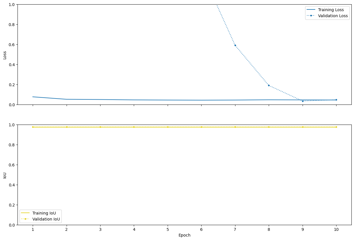

Learning curves

The training loss exhibits a clear downward trend, decreasing from approximately 0.08 to around 0.04 over the 10 epochs, indicating that the model is effectively learning and reducing error on the training dataset. The training IoU remains stable at about 0.97 throughout the process, while the validation IoU is consistently slightly higher at approximately 0.975, suggesting good generalization performance.

Although the validation loss shows some instability, particularly a very high value during the first epoch followed by fluctuations in subsequent epochs, it quickly stabilizes to low values, which may be attributed to initialization effects or data scaling issues rather than persistent model misfit. Overall, the model demonstrates strong and consistent segmentation performance.

Given these results, extending the training beyond 10 epochs may yield only marginal improvements. Considering the relatively small dataset, additional training could increase the risk of overfitting without significantly enhancing model performance.

3.3.4.3 Model evaluation

Now, we will use the test dataset, reserved for this moment. We can get the total metrics for the entire test data set.

evaluation = model.evaluate(
    x = testing_data,
    verbose = 1,
    steps = test_size
)

We can also apply the model to the test dataset, and graph the results.

prediction = model.predict(
    x = testing_data,
    verbose = 1,
    steps = test_size
)

By running the following code block we can visualize 3 random images from our test data set, and the model predictions.

np.random.seed(42)
n_images = 3

listTest = np.random.choice(test_size, size = n_images, replace = False)

print(listTest)

fig, axs = plt.subplots(n_images, 2, figsize = (15, 15))

for i in range(len(listTest)):
    imgTest = tf.math.divide(tf.squeeze(list(testing_data)[listTest[i]][0]), 12000)[:, :, 0:3].numpy()
    imgPred = prediction[listTest[i]].reshape(kernel_size, kernel_size)

    axs[i, 0].set_title('RGB Test Image ' + str(listTest[i]))
    axs[i, 0].imshow(imgTest)
    axs[i, 1].set_title('Prediction ' + str(listTest[i]))
    axs[i, 1].imshow(imgPred, cmap='coolwarm')

plt.subplots_adjust(wspace = -0.3, hspace = 0.4)
plt.show()

Despite being trained on a small dataset for only 10 epochs, the model produces high-quality segmentations with well-defined boundaries and contiguous regions, validating both the architecture choice and the training approach for this VHR satellite imagery application. This model proves that effective selective logging monitoring is achievable without massive datasets or extensive computational power. This modified U-Net architecture provides a powerful combination of high precision, data efficiency, and proven real-world effectiveness.

3.3.4.4 Save the model

Once we have an adequate model based on the metrics used, we will proceed to save it.

To do this we will use the tf.keras.save_model() function and we will have to specify the path to save the model.

# If necessary
!mkdir /content/drive/MyDrive/DL_Book/model/

modelDir = '/content/drive/MyDrive/DL_Book/model/logging_model.keras'
tf.keras.models.save_model(model, modelDir)

In the next section, we will load our model again and apply it to the whole image!

3.4 Part III: Model application

This section demonstrates the workflow used to apply our deep learning model locally, which was trained and saved in the previous section (Part II). We will load the trained U-Net model, as well as our SkySat image. We will split the image into patches and apply the model to each patch separately. Finally, we will merge all the fragments and resynthesize the image. This workflow is designed for use in Google Colab.

This section will require the following packages:

• TensorFlow.
• Numpy.
• GDAL.
• Google Drive.
• Matplotlib.

We will again import the TensorFlow library, to load our model and apply it.

import tensorflow as tf
print(tf.__version__)

Also, Numpy for manipulating the tensors (patches). Note that TensorFlow has many built-in functions that have the same capabilities as Numpy. However, this notebook will use Numpy.

import numpy as np

GDAL is also a fundamental library, that allows us to save, export and manipulate rasters. It is also used in QGIS in many tools. Note that there are other libraries that can read satellite images such as Rasterio and Rioxarray. However, GDAL is a core library that is used as a backend by these more modern packages.

from osgeo import gdal

Again, we will link our notebook with Google Drive. Note that there are different platforms to store models, such as Hugging Face. However, we will work with Google Drive for its practicality.

from google.colab import drive
drive.mount('/content/drive')

And finally, import Matplotlib for the visualization.

import matplotlib.pyplot as plt

If you do not wish to run the previous section, you can create a copy from the original folder. Click here to go to the Drive folder. Make sure to modify the paths to match the current notebook.

3.4.1 Model loading

If you have followed the previous steps, you will have your model stored already in Google Drive, we will load our model with the tf.keras.models.load_model() function.

modelDir = '/content/drive/MyDrive/DL_Book/model/logging_model.keras'
model = tf.keras.models.load_model(modelDir)

We can visualize the structure of our loaded model and the amount of parameters in each layer.

model.summary()

Next, we will download a very-high resolution image from SkySat (0.5 m), we will use the wget linux command.

!wget --no-check-certificate 'https://raw.githubusercontent.com/NASA-EarthRISE/EarthRISE-Applied-Artificial-Intelligence-and-Deep-Learning-Book/main/03_Semantic_Segmentation/02__Selective_Logging_Detection/img/Skysat_20201017_ssc2_150055_COG_clip.tif' -O Skysat_20201017_ssc2_150055_COG_clip.tif

Let’s visualize the downloaded image!

img_path = 'Skysat_20201017_ssc2_150055_COG_clip.tif'
img_to_viz = gdal.Open(img_path, gdal.GA_ReadOnly)

img_array_viz = img_to_viz.ReadAsArray().transpose([1, 2, 0])
rgb_img = np.divide(np.stack([img_array_viz[:,:,2], img_array_viz[:,:,1], img_array_viz[:,:,0]]), 12000.0)

plt.figure(figsize=(10, 10))
plt.imshow(rgb_img.transpose(1, 2, 0))
plt.title('Downloaded SkySat Image (RGB)')
plt.axis('off')
plt.show()

del img_to_viz

This satellite image was taken from an indigenous community called Fatima in the year 2021. In this community, more than 300 trees were detected being cut down. Imagine how long it would take a GIS specialist to gather data through manual digitization. We will apply the already trained model to the image and analyze the output of the model.

3.4.2 Model application

We will define the input path of our image, and the desired output path.

img_path = 'Skysat_20201017_ssc2_150055_COG_clip.tif'
out_path = 'Skysat_20201017_ssc2_150055_COG_pred.tif'

With gdal.Open() we can get important details about our image and use the GDAL python API.

img = gdal.Open(img_path, gdal.GA_ReadOnly)

We are interested in the pixel values, so we will read the image as an array. Since GDAL returns the image with the structure (Bands, Height, Width), we will transpose our image to the following structure (Height, Width, Bands).

img_array = img.ReadAsArray().transpose([1, 2, 0])
print(img_array.shape)

Since our model is object-based, it operates according to patches, and our image must match its input size (in this case 128 by 128). We will add a zero padding to the borders of our image, to have compatible patch sizes. The following code calculates the amount of rows and columns to add with the 0 padding.

print('rows (heigth) to add with 0: ', 128 - img_array.shape[0] % 128)
print('cols (width) to add with 0: ', 128 - img_array.shape[1] % 128)

This block of code will create a zero row padding, and append it to the original image.

row_padding = np.zeros([128 - img_array.shape[0] % 128, img_array.shape[1], img_array.shape[2]])
img_rdy = np.append(img_array, row_padding, axis = 0)
img_rdy.shape

This will add a zero column padding. Notice that the final size of the image is entirely divisible by the patch size (128).

col_padding = np.zeros([img_rdy.shape[0], 128 - img_array.shape[1] % 128, img_array.shape[2]])
img_rdy = np.append(img_rdy, col_padding, axis = 1)
img_rdy.shape

We will use some functions of the Patchify library. To extract patches of equal size from our input image, this function uses Numpy.

# Patchification
def patchification(arr_in, window_shape, step = 1):

    # Dimensions of the input array
    ndim = arr_in.ndim

    # Step multiplied the amount of dimensions
    step = (step,) * ndim

    # Create a sliding window
    slices = tuple(slice(None, None, st) for st in step)

    # Obtain the strides of the input array
    window_strides = np.array(arr_in.strides)

    # Obtain the strides of the moving window applied to the input array
    indexing_strides = arr_in[slices].strides

    # Generate a shape with the amount of patches per row and column
    win_indices_shape = (
        (np.array(arr_in.shape) - np.array(window_shape)) // np.array(step)
    ) + 1

    # Generate the final shape of the output
    new_shape = tuple(list(win_indices_shape) + list(window_shape))

    # Merge the strides of the index and window
    strides = tuple(list(indexing_strides) + list(window_strides))

    # Obtain the patches
    arr_out = np.lib.stride_tricks.as_strided(arr_in, shape = new_shape, strides = strides)
    return arr_out

This block of code uses the previously created function to extract our patches. Notice that by using .reshape() we are concatenating each patch and now we have an extra dimesion. Our structure now is (Batch, Height, Width, Band). In this case, the batch is the number of patches on which the model will be applied.

patches = patchification(img_rdy, [128, 128, 4], 128) \
    .reshape([int((img_rdy.shape[0] * img_rdy.shape[1]) / (128 * 128)), 128, 128, 4])
patches.shape

Finally, we apply our model to our structured patches.

# Apply the model on the processed array
predictions = model.predict(patches, verbose = 1)

We will create another function, that unpatchifies our predictions.

# Function to merge the patches
def unpatchification(arr_in, window_shape, height, width):
    result_array = np.empty([img_rdy.shape[0], img_rdy.shape[1], 1])
    row = 0
    col = 0
    for patch in arr_in:
        result_array[window_shape[0] * row : window_shape[0] * (row + 1), window_shape[1] * col : window_shape[1] * (col + 1), :] = patch
        col += 1

        if (window_shape[1] * col) == width:
            row += 1
            col = 0
    return result_array

Notice the .transpose() function, that will restore the original shape used by GDAL (Band, Width, Height).

# The predictions must be reshaped to the same dimensions of the input image
final = unpatchification(predictions, [128, 128], img_rdy.shape[0], img_rdy.shape[1]).transpose([2, 0, 1])
final = final[:, 0 : img_array.shape[0], 0 : img_array.shape[1]]
final.shape

Finally, we will load our predictions, and register its metadata to GDAL. The most important aspect in this step is the projection. It must match the input image. Otherwise, our image won’t have a location in the space.

# Now we will register a new image using GDAL
driver = gdal.GetDriverByName('GTiff')
driver.Register()

# We'll use the shapes of the output
outDataset = driver.Create(out_path, final.shape[2], final.shape[1], final.shape[0], gdal.GDT_Float32)
outDataset.SetProjection(img.GetProjection())
outDataset.SetGeoTransform(img.GetGeoTransform())
outDataset.GetRasterBand(1).WriteArray(final[0, :, :], 0, 0)

del outDataset

We can visualize our predictions and the input image.

fig, axs = plt.subplots(1, 2, figsize = (25, 25))

axs[0].set_title('RGB Image')
axs[0].imshow(np.transpose(np.divide(np.stack([img_rdy[:,:,2], img_rdy[:,:,1], img_rdy[:,:,0]]), 12000), [1, 2, 0]))

axs[1].set_title('Prediction')
axs[1].imshow(final[0, :, :])

plt.show()

Detection of selective logging using the trained model

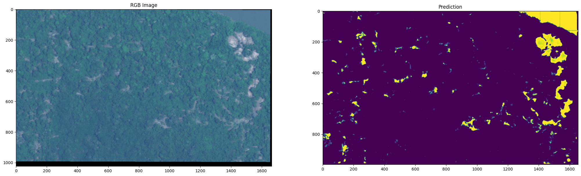
As you can see, models are not perfect. There are some artifacts that affect our predictions. There are subtle vertical and horizontal lines creating a grid pattern across the entire prediction. This is because the model sees each patch independently without context of adjacent areas. There are also features that span tile boundaries and get processed differently on each side. There are advanced techniques to solve this, such as creating an overlap-tile strategy. This means processing patches with 50% overlap and blend the output. Another way to solve this would be through weighted averaging, which is giving more weight to center of patches, and less to edges.

3.4.3 Discussion

We have successfully applied our model to a scene from a SkySat image. Through visual inspection, we can see that the model isn’t perfect. In fact, it confuses water with selective logging. This is possibly due to the limited amount of data containing water as a background. Another interesting effect is the edge effect. You can see in the upper right corner of the predictions that there are lines with low probability. This can be corrected by overlapping patches.

To evaluate the effectiveness of the model, validation is necessary. There are different validation techniques, with numerous types of sampling. However, this notebook will not address these topics as they are subjective, in line with the study objective.

We encourage you to make changes to these notebooks, configure hyperparameters, patch size, batch size, learning rate, epochs, among others.

3.4.4 Optional - cleaning your folder

Use the following code to clean the contents of your folder.

#!rm -rf /content/drive/MyDrive/DL_Book/*

You can also do it manually in Google Drive.