10.2 Earth Observation Foundation Models: Encoder Representation Analysis and Downstream Task Benchmarking
Authors
Affiliations

Ryan P. DeMilt

Spatial Informatics Group

Nicholas LaHaye

Jet Propulsion Laboratory

Spatial Informatics Group

Myscon Truong

Spatial Informatics Group

Karis Tenneson

Spatial Informatics Group

David Saah

University of San Francisco

Spatial Informatics Group

Open in Colab Run in Colab View on GitHub View on GitHub

* Ryan P. DeMilt, Nicholas LaHaye, and Myscon Truong contributed equally to this work.

How to cite this chapter:

DeMilt, R. P., LaHaye, N., Truong, M., Tenneson, K., & Saah, D. (2026). Earth Observation Foundation Models: Encoder Representation Analysis and Downstream Task Benchmarking. Zenodo. https://doi.org/10.5281/zenodo.23001198 DOI

Part of: Mayer, T., Bhandari, B., & Saah, D. (2026). EarthRISE Applied Artificial Intelligence and Deep Learning Book. Zenodo. https://doi.org/10.5281/zenodo.20547796 DOI

Overview

This chapter explores how to inter-compare different Earth Observation Foundation Models’ requirements, behavior, and performance on two related wildfire monitoring tasks.

Before getting started, let’s first walk through setting up the Python environment, installing the necessary frameworks, and downloading the datasets so that all subsequent analyses can run end-to-end without additional configuration.

Software/Hardware considerations

CUDA is NVIDIA’s parallel computing platform and software stack for running general-purpose code on NVIDIA GPUs. While it is not necessary, we recommend running this notebook in a CUDA-enabled Linux environment for convenience and ease of setup. We have tested this notebook using Google Colab’s “Latest” runtime environment (v2026.04) and a T4 GPU, which is available under Colab’s free tier.

We handle environment setup below, defaulting to a setup that works within Colab. If you choose to alter the environment or run elsewhere, the authors recommend installing Python >= 3.10 either standalone or through a conda-managed environment. To estimate the VRAM required for storing the model, we can use a simple calculation of # of parameters and precision. For example, a 300M parameter model at 32bit precision would roughly require 3.6GB to store the weights and optimizer states. Another 1.2 GB is required for the gradients of each of those parameters and a few more for the data itself. Likewise, the decoder used to extract from the internal representation also imposes VRAM / compute requirements. There’s no universal formula here, but tools like PyTorch hooks, torch.cuda.memory_summary(), or profilers can help estimate how much compute you need. 12GB of VRAM is a good place to start, and luckily there are free Google Colab options at this compute scale, but there is a trend towards larger and more complex models, which inevitably consume more compute.

Timing considerations

Here we provide time estimates for all examples run in the notebook. We break it down into sub-categories of tasks that are sequentially dependent on one another. With this information, you can choose to run through different examples separately, without worrying about missing dependencies, etc.

Note that all of these sub-categories are dependent on the environment setup and data downloading.

Runtimes: - Environment setup and data download: 15 minutes - Weight matrix analysis: 30 minutes - Model resource requirement computations: 1 minute - Embedding analysis: 3 hours and 25 minutes - Embedding generation: 5 minutes - KNN graph generation: 1 hour - Data kernel analysis: 2 hours and 20 minutes

  • Model training and task evaluation (HLS Burnscars): 4 hours

  • Model training and task evaluation (MTBS): 8 hours

We are installing directly from cloned repos along with the available requirements.txt file. This may take a few moments as PyTorch is a fairly large package. If not using Colab, please install Python and pip on your own and set up your notebook environment that best suits your preferences.

Logging and Model Examination

Weights & Biases (WandB) is a popular tool for experiment tracking, model monitoring, and collaboration in machine learning workflows. It integrates seamlessly with PyTorch, TensorFlow, Keras, and other frameworks, allowing users to log training metrics, visualize results in real-time, and compare model performance across runs. Pangaea benchmark has a pre-baked integration with WandB that is easily accessed using WandB’s API key authentication protocol. We have set up all script runs that provide WandB utilization options to run without an account by setting the environment variable WANDB_MODE=offline.

This is optional, but if you would like to learn more about creating an account and interfacing with WandB, see WandB documentation on environment variables and account creation.

Environment Setup

The next few cells set up the environment and pull the necessary data for the chapter’s examples.

Show code
from google.colab import drive

drive.mount('/content/drive')

!cd /content/
!git clone --branch "eofm_book_0.2" --single-branch https://github.com/sig-gis/pangaea-bench.git
!pip install -e "pangaea-bench"
!pip install -r pangaea-bench/requirements.txt

!git clone --branch v0.1 --single-branch https://github.com/sig-gis/calculate-flops.pytorch.git

!export PYTHONPATH=${PYTHONPATH}:/content/calculate-flops.pytorch/
Show code

from pydrive2.auth import GoogleAuth
from pydrive2.drive import GoogleDrive
from google.colab import auth
from oauth2client.client import GoogleCredentials

#CROMA weights and datasets are large and sometimes fail to download automatically.
#Ensuring we have them by manually downloading here.
!mkdir -p /content/pangaea-bench/pangaea/encoder_analysis/pretrained_models/
!mkdir /content/data/
!ln -s /content/data/ /content/pangaea-bench/pangaea/encoder_analysis/

#CROMA weights
!wget https://huggingface.co/antofuller/CROMA/resolve/main/CROMA_large.pt -O /content/pangaea-bench/pangaea/encoder_analysis/pretrained_models/CROMA_large.pt

#HLS Burnscars Dataset
!wget https://huggingface.co/datasets/ibm-nasa-geospatial/hls_burn_scars/resolve/main/hls_burn_scars.tar.gz -O /content/data/hls_burn_scars.tar.gz
%pushd /content/data/
!mkdir ./hlsburnscars/
!tar -xf hls_burn_scars.tar.gz -C ./hlsburnscars/

#MTBS Dataset
auth.authenticate_user()
gauth = GoogleAuth()
gauth.credentials = GoogleCredentials.get_application_default()
drive = GoogleDrive(gauth)
downloaded = drive.CreateFile({'id': '1zZzEypFPxjirBUtHU_T4IEBwq9vMZq6k'})
downloaded.GetContentFile("mtbs_fires.zip")

!mkdir /content/data/mtbs/
!mv mtbs_fires.zip /content/data/mtbs/
%pushd /content/data/mtbs/
!unzip mtbs_fires.zip
%popd

%popd
Show code
#Move to directory.
#This directory will be used for all subsequent encoder analysis tasks as well.
%pushd /content/pangaea-bench/pangaea/encoder_analysis/

#Library writes to local directories.
!mkdir img
!mkdir ww-img
!mkdir -p ww/croma/
!mkdir -p ww/dofa/
!mkdir -p ww/prithvi/
!mkdir ./embeddings/

Section A: Introduction

Scientific Background and Problem Formulation

In this notebook, we will be exploring adapting Earth Observation Foundation Models (EOFMs) to a pair of wildfire monitoring tasks. To begin, we will discuss the tasks, the associated challenges, and the utility that emerging techniques may have to offer. Our goal in this chapter is to walk through these ideas step by step, assuming only a basic familiarity with machine learning and remote sensing.

Problem Formulation

Following a wildfire event, it is vital to assign resources to determine the extent of the damage caused to people, their properties, and the environment, and the depth of the long-term effects of the event. This can be done through examining remotely sensed Earth observation data, such as Sentinel-2 imagery. However, these assessments can be time-consuming and expensive to produce.

The work is traditionally done using hand-tuned thresholds for specific indices such as NBR (Normalized Burn Ratio) and dNBR (delta Normalized Burn Ratio) (Cocke et al., 2005; Roy et al., 2005). These thresholds are then specific to the regions they are developed for, sometimes even specific to a single event, and require expert knowledge to produce. This leaves these assessments inaccessible to many who lack the resources and access to expertise required for their generation, creating many barriers which make the prospect of automation attractive for these tasks.

More traditional data-driven approaches, such as supervised learning methods, may still impose significant requirements of large labeled datasets and custom architecture development. With EOFMs, pretrained using self-supervision, comes the hope that models will learn generalizable features from large collections of unlabeled data whose insights can then be transferred to a wide array of specific tasks. This is connected to the hope that fine-tuning these models will be more straightforward than traditional methods, thereby reducing duplication of effort and costly model training time.

Here we will examine two tasks related to the wildland fire severity assessment context described above: mapping burn scars and mapping burn severity. In both cases, we work with optical satellite imagery and associated labels. The datasets we will use are:

  • HLS Burn Scars: The HLS Burn Scars dataset (Phillips et al., 2023) consists of paired Harmonized Landsat–Sentinel (HLS) images and corresponding burn scar masks from 2018–2021 over the contiguous United States. The input imagery is continuous reflectance data across multiple spectral bands, and the labels are binary masks indicating burned vs. unburned pixels for each scene. These masks are derived for individual fire events. This structure makes the dataset well suited for semantic segmentation and for studying how encoders separate burned and unburned classes in embedding space.

  • Monitoring Trends in Burn Severity (MTBS): The MTBS project uses expert-driven interpretation of pre‑ and post‑fire imagery to assign categorical burn severity classes (e.g., unburned/low, moderate, high) within mapped fire perimeters. In our setup, we pair these discrete severity labels with Landsat-based optical imagery collected before and after fire events. As with the HLS Burn Scars dataset, the input data are continuous reflectance values, but here the targets are multi-class severity labels. The temporal baseline is again event-centered: images are selected relative to each fire’s occurrence to capture pre‑ and post‑fire conditions. This combination of continuous imagery and categorical severity classes provides a way to test how different encoders structure severity gradients in their embedding spaces, and how well various decoders can recover those distinctions.

As we make decisions on utilizing and adapting existing foundation models to these tasks, many questions arise, including:

  • What do we need to do to adapt our EOFMs to these tasks? What are the downstream impacts of these decisions on performance and usability of our final solution?
  • Which models perform the best on our task? How do we compare them to each other and to our possible baseline methods?

Underlying all of these practical questions are more abstract questions regarding the validity of these models and why they behave the way they do. We will discuss these concepts in detail in this tutorial, using the aforementioned post-fire monitoring problems as a frame to help the reader develop an understanding of these topics and apply them to their use cases. Because EOFMs are still rapidly evolving, many topics we touch on remain open research questions, and the material here will continue to change as the associated fields progress. We aim to provide a snapshot of the situation as it stands, as well as commentary to help frame discussion on how to approach these open topics and equip our readers to confront them.

To do that, we first introduce a few core ideas from modern deep learning, including transfer learning, foundation models, and embeddings, and connect them to the wildfire tasks described above.

Technical Background and Introduction

Transfer Learning and Beyond

Transfer learning is a powerful machine learning technique that allows a model trained on one task to leverage previously learned features for a different but related task. Instead of starting from scratch, transfer learning leverages the knowledge a model has already gained from a separate, and usually large, dataset and applies it to a new problem. This is particularly useful when a dataset is small or annotations for the new task are limited. Once initial training has been completed, the layers toward the front (closer to the input layer) of these models have typically learned general features, such as edges in images or syntactic patterns in text, which can be useful across a wide range of tasks.

Ideally, by fine-tuning the initial layers of a pretrained model or adding new layers specific to the new task, practitioners can adapt it to perform well with far fewer training samples. This also has the potential to improve performance thresholds for a given smaller or imbalanced dataset, as the pretrained model already has latent feature extraction capabilities from prior training. Properly executed transfer learning not only has the potential to boost performance, but also saves computational resources and significantly reduces training time. You can think of this as skill reuse: a model that has already learned to recognize generic shapes and textures in one dataset can adapt more quickly to a new dataset.

Many different strategies can be applied to achieve transfer learning, such as freezing different sets of layers during training or allowing all layers to be updated, depending on the similarity between the source (initial) and target (new) tasks. For example, in medical imaging, models trained on natural images have been fine-tuned to detect tumors or classify X-rays by retraining only a few layers.

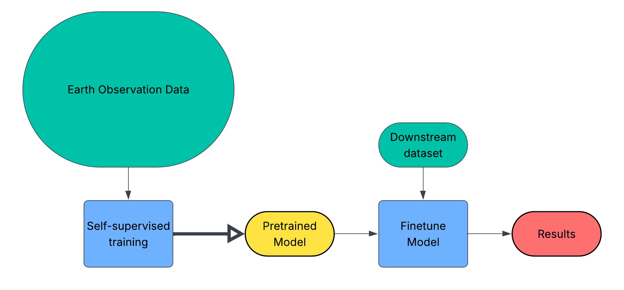
Diagram of a foundation model pretraining workflow feeding into downstream tasks

Diagram of a foundation model pretraining workflow feeding into downstream tasks
Figure 1. Simplified foundation model pretraining workflow


An emerging category of models, termed ’ Foundation Models’ (FMs), uses transfer learning at a much larger scale. Here, we use the term ‘foundation models’ to refer specifically to large, pretrained neural networks—typically deep encoders, such as Convolutional Neural Networks or Vision Transformers, trained on massive, unlabeled Earth observation datasets, with the goal of learning general-purpose representations (Bommasani et al., 2021). Within the training and architectural paradigms for these models, the pretraining task is designed to learn general-purpose representations from a large unlabeled collection of data. These representations can then serve as the foundation for many different models and downstream tasks (Figure 1). This contrasts with traditional supervised learning problems that aim to map data samples to annotations from a specific task. FMs are said to be trained in a ‘self-supervised’ manner and potentially offer similar benefits to models developed using traditional transfer learning techniques (i.e reduced training time and improved performance). However, unlike with transfer learning, FMs circumvent the development of an initial large-scale labeled dataset. This technique is especially powerful in the remote sensing world where the availability of large-scale unprocessed data is ever-increasing, and the methods for transforming it into actionable insights draw from a wide range of scientific disciplines. The larger goal of the EOFM development communitity is to create models capable of generalizing across Earth Science domains and remote sensing modalities by learning from the structure and correlations inherent in the raw data, and enabling a wider array of practitioners, and more versatile models to adapt them with minimal fine-tuning. Attempts towards this ephemeral goal, however, must be thoroughly assessed in a way that adheres not just to typical computer vision analysis, but also to the rigor required with respect to both the underlying science goals and the remote sensing instrumentation (DeMilt et al., 2025).

If truly foundational, a foundation model plays a similar role to a good set of “starter features” that many different teams can build on. Instead of each project training a model from scratch, a single, large encoder can be adapted to many downstream tasks, including regression, segmentation, and change detection, by adding relatively small task-specific components on top. We refer to these small supplementary models as “decoder heads”. Their job is to customize our pretrained foundation model to complete our task.

In the next few subsections, we briefly survey how these encoders are pretrained. It is not required to master all of the details of each method, but we want to provide enough context to help build intuition and depth of interpretation for use later in the chapter.

Pretraining Methodologies

Below are three categories of methods for pretraining a computer vision model in a self-supervised fashion. These methods have been combined and extended in many ways to create the present field of EOFMs. This list is not exhaustive, as widespread satellite data access has led to many variations and combinations, as well as other less commonly used techniques. There is also extensive effort to connect strides made separately within the computer vision and natural language processing domains, both within and beyond the remote sensing community.

It is worth noting that the models described and tested here are all transformer-based, where the core architectural unit is a vision-transformer trained under the ‘encoder-decoder’ paradigm (to be discussed) (Vaswani et al., 2017; Kolesnikov et al., 2021). While it is important to understand the high-level distinction between these techniques, it is not entirely necessary to implement them in practice, as many developer groups have worked hard to abstract most of the logic away in various frameworks (Han et al., 2022). Deep understanding of each of these model families, as well as the nuances of transformer architectures, is beyond the scope of this chapter, and not strictly necessary to benefit from the material here. We encourage interested readers to explore these topics further, but our focus will be on the main ideas and how to use them in practice. The deeper a practitioner’s knowledge, the easier it will be to distinguish between appropriate and inappropriate practices both with data and the associated model training and deployment.

Masked Autoencoding (MAE)

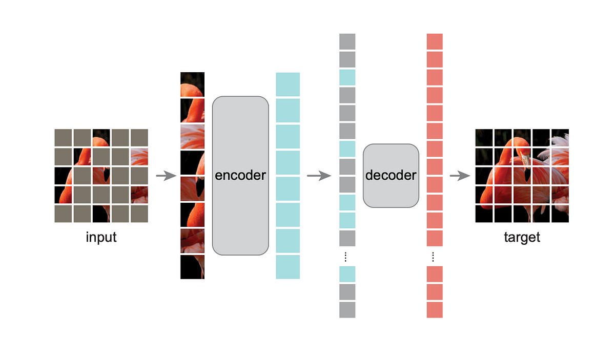
Masked autoencoder diagram showing image patches masked and reconstructed by a decoder

Masked autoencoder diagram showing image patches masked and reconstructed by a decoder
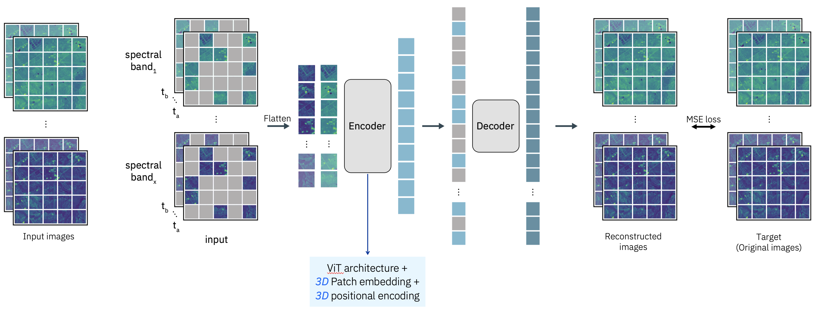
Figure 2. Diagram depicting masked autoencoder training from (He et al., 2022). Images are broken into small sections, called patches. A percentage of these patches are hidden (masked). The decoder is tasked with reconstructing the original image from the remaining unmasked patches.


Autoencoder-centric methods consist of an encoder that projects input images into a (typically) lower-dimensional latent (or embedding) space and a decoder that reconstructs the original images from these representations. This compression helps the model capture essential features while discarding noise or irrelevant details. By reconstructing lost information with remaining unmasked patches, models are expected to encode general image features and develop image-level understanding and fine-grained spatial reasoning. This process is sometimes referred to as masked image modeling (MIM). Masked tokens do not have to be processed by the encoder, as they are effectively ignored. Higher masking levels therefore reduce computation per sample, which can be traded for more training iterations or larger datasets (He et al., 2022). Figure 2 depicts the masked autoencoder training flow.

Contrastive Learning

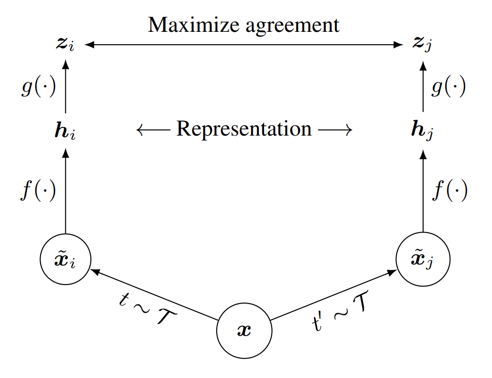
SimCLR contrastive learning diagram showing augmented image pairs and embeddings

SimCLR contrastive learning diagram showing augmented image pairs and embeddings
Figure 3. Diagram for SimCLR training paradigm from (Chen et al., 2020).


Contrastive models are tasked with distinguishing between similar and dissimilar image representations. They do this by pulling together representations of positive pairs (different augmented views of the same sample) so that they lie close to one another in the model’s embedding space, while pushing dissimilar pairs farther apart, typically using views from different images. An example flow diagram can be seen in Figure 3. Common methods include Simple Contrastive Learning (SimCLR) and Momentum Contrast (MoCo) (Chen et al., 2020; He et al., 2020).

In this setting, and the broader context of deep learning, an embedding is a vector representation produced by the encoder for each sample (here, an image or image patch). Informally, you can think of an embedding as the model’s internal summary of an input sample: a list of values that captures which patterns, colors, and shapes it considers most important for distinguishing one scene from another. The contrastive loss operates directly on these vectors or lists, shaping the geometry of the latent space so that samples deemed similar by the training signal occupy nearby regions, and dissimilar samples are separated. Unlike with masked autoencoders, a decoder is typically not included in the pretraining phase, since the task is defined entirely in this latent space rather than in the pixel space of the original image.

This methodology usually requires some level of annotation or at least a notion of correspondence, for example by defining positive and negative pairs within the training data, and can sometimes be referred to as a semi-supervised methodology. The resulting training objective tends to produce embedding spaces with stronger, more explicit notions of similarity: clusters or manifolds that reflect semantic or physical relationships between samples. This, in turn, leads to latent space properties that can differ substantially from those of masked autoencoder models.

Non-contrastive Self Distillation

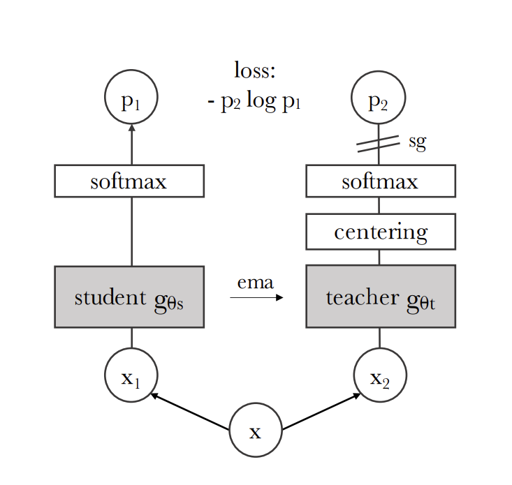
DINO self-distillation diagram with student and teacher networks processing augmented views

DINO self-distillation diagram with student and teacher networks processing augmented views
Figure 4. Diagram for DINO training paradigm from (Caron et al., 2021).


Non-contrastive self-distillation is a self-supervised learning approach for computer vision that avoids the need for negative samples. Instead of contrasting different images, it trains a student network to match the output of a teacher network, both fed with different augmented views of the same image. The teacher is often an exponential moving average of the student, meaning that it is a slowly changing average of student models. This provides stable targets for the two encoders while distilling knowledge from the teacher model. Figure 4 shows an example of this approach. The objective is to produce consistent, meaningful embeddings, not to reconstruct or generate the input. Common methods include ‘Self-distillation with no labels’ (DINO) and ‘Bootstrap Your Own Latent’ (BYOL) (Grill et al., 2020; Caron et al., 2021). These methods are often combined with different pretraining objectives and are a strong method for refining new models while utilizing the results of existing ones.

Decoders

Just as you would with any trained neural network, you can load the weights for inference using similar code you might have seen in previous chapters. There is still one more consideration you must make depending on the type of task at hand and the shape of the encoder’s output. If your goal is to classify images, a lightweight machine learning algorithm directly on top of the embedding vector outputs of the encoders may be sufficient. The assumption here is that the model’s internal representation of the image is robust and relevant to your task. We will touch on this topic below. If your goal, on the other hand, is to segment the images, we may need to train a subsequent neural network to extract from that internal representation and produce a fine-grained map. Below is a summarization of contemporary decoder types commonly used in conjunction with transformer-based encoders. Each varies in complexity, purpose, and the method by which it extracts features from the transformer layers in the aforementioned encoders.

Linear Probe

Diagram of a simple linear probe decoder with a single linear layer

Diagram of a simple linear probe decoder with a single linear layer
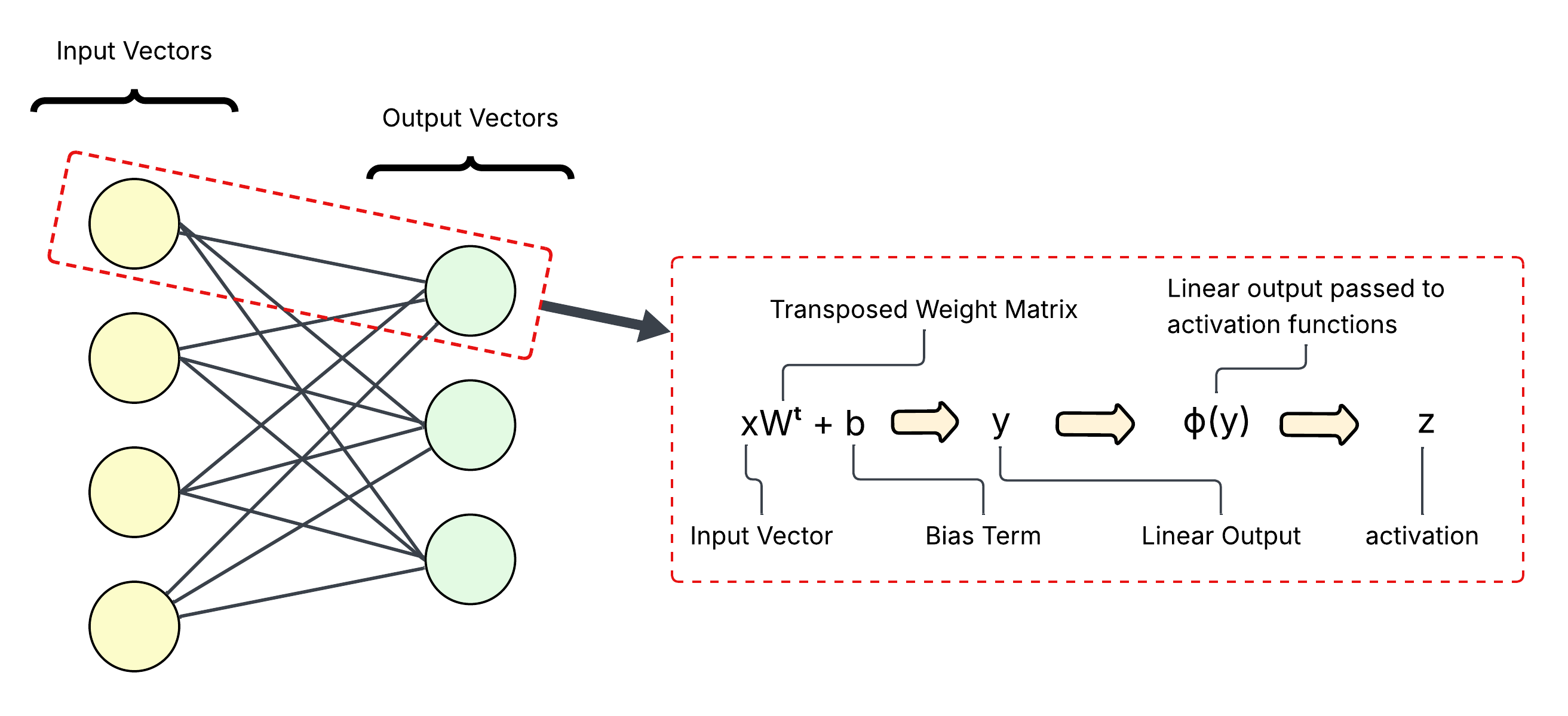
Figure 5. Simplified structure of a single linear layer.


A linear probe, as displayed in Figure 5, is the simplest type of decoder typically used in this paradigm. It is a single linear layer, or a small multi-layer perceptron (MLP). This technique is taken from the language domain where large language models are often evaluated on downstream tasks with linear probes on frozen embeddings before doing full fine-tuning. In practice, this isn’t typically used for many Earth observation tasks due to limited model complexity. But this decoder is still useful in assessing representation quality as it is cheap to train and can be implemented consistently, making it an ideal tool for benchmarking. Since the model is so simple, the performance of a linear decoder can be used to analyze how easily separable the encoder has made the samples from our dataset.

Fully Convolutional Network (FCN)

Fully convolutional network architecture diagram with stacked convolutional layers

Fully convolutional network architecture diagram with stacked convolutional layers
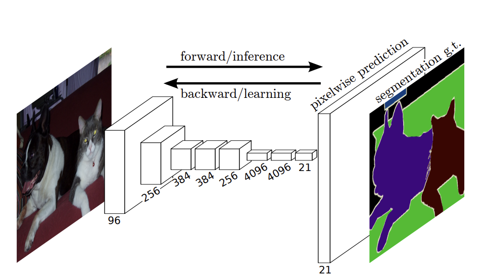
Figure 6. Full convolutional neural network architectural diagram from (Long et al., 2014).


The FCN, shown in Figure 6, is a stack of convolutional layers that upsample and refine the final feature maps produced by the transformer’s output embeddings, converting them back into an image-like spatial representation. This final representation can then be fed through a final prediction layer, which is typically itself a set of convolutional layers, to produce the final map (Long et al., 2014). This is typically more lightweight than some of the MLP-based decoders below, due to weight sharing in the learned convolutional kernels. Local context is also explicitly emphasized as those same kernels typically only cover a small portion of the whole input image at a given time.

SegFormer

SegFormer architecture diagram for semantic segmentation with a lightweight decoder

SegFormer architecture diagram for semantic segmentation with a lightweight decoder
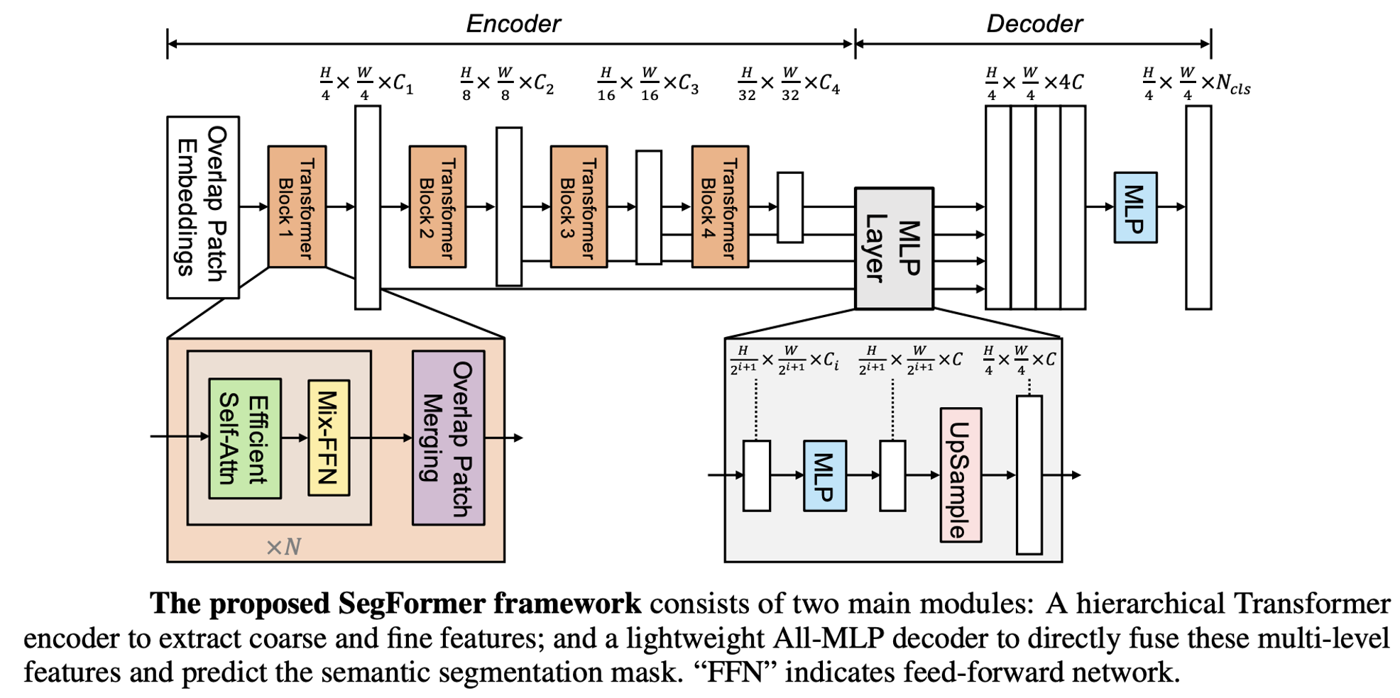
Figure 7. SegFormer-style network architectural diagram for semantic segmentation from (Xie et al., 2021).


SegFormers use an MLP-style decoder to extract information from a set of hierarchical features taken from transformer-based encoders (Xie et al., 2021). An example is shown in Figure 7. Originally developed as a standalone framework for end-to-end training, SegFormer has recently been adapted by a handful of research groups attempting to utilize the representation generated by the pretraining phase in this same way. The assumption is that the implementation of the transformer blocks in the encoder is sufficiently hierarchical in nature such that they can be composed using this method.

UperNet

UperNet architecture diagram showing multi-scale hierarchical feature pooling

UperNet architecture diagram showing multi-scale hierarchical feature pooling
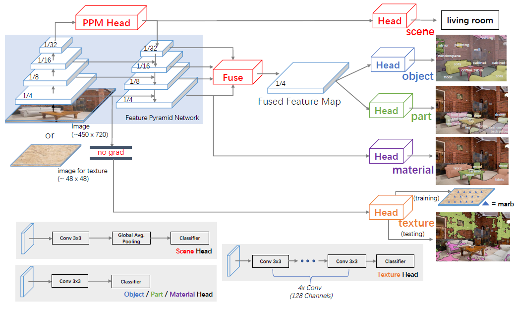
Figure 8. UperNet architectural diagram from (Xiao et al., 2018).


Similar to the SegFormer architecture, the UperNet leverages multi-scale hierarchical features to generate dense (per-pixel) predictions. Rather than MLPs, the UperNet utilizes pooling layers and convolutions to compose the features before the final prediction layers. An example of UperNet can be seen in Figure 8. It’s worth noting here that the original UperNet use case used a fine-tuned ResNet-50 backbone. In other words, this architecture has been closely aligned with the ‘pretrained encoder’ / decoder paradigm that has been popularized in the last few years (Xiao et al., 2018).

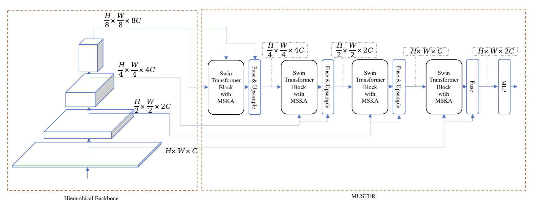
MUSTER

MUSTER decoder architecture diagram showing transformer-based hierarchical feature extraction

MUSTER decoder architecture diagram showing transformer-based hierarchical feature extraction
Figure 9. Architectural diagram of MUSTER decoder from (Xu et al., 2022).


MUSTER, as seen in Figure 9, is a more recent decoder development in the computer vision realm. Similar to both the SegFormer and the UperNet. Hierarchical features play an important role in its predictive strength, with the most important distinction here being that the decoder itself is also transformer-based (Xu et al., 2022). Also similar to the UperNet, the MUSTER decoder was designed to integrate with pretrained encoders. While this may lend itself to greater performance, it is important to consider the compute required to implement such an architecture.

Encoder Evaluation

When working with EOFMs, it is not enough to evaluate only the final task performance. We also need to understand how well the encoder itself represents the data. This process requires a multifaceted approach on both the data and analysis fronts. Because an encoder model is meant to have broad purpose and applicability, no single metric or dataset is sufficient to understand the model’s performance and utility for downstream users. For a beginner, it may help to think of this as stress-testing the encoder: on top of understanding if a model performs well on a given task or benchmark, we want to understand how it behaves under different data conditions, what kinds of patterns it tends to learn, and what the computational and environmental cost of training and deploying various solutions is.

Despite this complexity, there are common factors to consider. Diversity of datasets, which can cover broad conceptual categories within the fields of remote sensing and Earth system science, is an important factor. While no dataset is the perfect exemplar, a dataset similar to the one a given model was pretrained on may give an initial assessment of a model’s applicability to a new task. Diverse training and inference settings are equally important. Understanding a model’s performance in many settings such as varying image sizes, geographic regions, and spatial scales can reveal strengths and weaknesses of each encoder. It can enlighten both the downstream user and the researcher looking to improve their encoder.

While this chapter is not focused on dataset accumulation, it should also be mentioned that proper splitting of the data in a geospatial setting is imperative for proper evaluation and should consider variables like keeping unseen spatiotemporal areas as a held-out test set for independent post-training evaluation of a model. This ensures that complex spatiotemporal cues built into geospatial datasets are not “memorized” and overstate a model’s performance on a given task and potential generalizability (LaHaye et al., 2021; Parajuli et al., 2024). Here we discuss some ways an encoder’s representational “skill” can be measured and evaluated by looking at both the model’s weight matrix and its embedding vectors. Unlike the metrics used for downstream task evaluation, many of these are newer and therefore less well-known. Here we provide a brief description and references for each methodology used.

Resource Requirements

In this section, we introduce simple proxies for resource requirements of a given model (Floating Point Operations (FLOPs), Multiply-Accumulate Operations (MACs), and parameter counts) that help you estimate whether a model will fit your hardware and runtime constraints. As data science practitioners, we typically want to balance performance, interpretability, and resource requirements as three main driving factors in model selection. It is also crucial that we aim to choose the smallest and most efficient model that meets the requirements for our task in these three areas. This is important not only for efficiency, but also because the environmental impact of large-scale deep learning models has become a significant concern as model sizes and computational demands continue to grow. Choosing small and optimized models where appropriate is an effective strategy for reducing the emissions and energy consumption footprint associated with model development and deployment (Strubell et al., 2019; Patterson et al., 2021) . These considerations should also include a model’s pretraining phase as well as resources required for fine-tuning and operational inference.

FLOPs, MACs, and parameter counts are three metrics that offer practical proxies for estimating a model’s resource requirements. FLOPs denote the total number of floating-point operations (additions, multiplications, etc.) required to process a single input through the model. High FLOPs indicate a model that requires substantial computation resources, which can translate directly to longer inference and training times. Multiply-accumulate operations, foundational to neural network layers (especially in convolutions and matrix multiplications), are closely linked to the physical operations that deep learning accelerators (like GPUs and TPUs) execute, providing an estimate of the actual computational workload. The parameter count measures the total number of learnable variables (weights and biases) within a model. The number of parameters is a large driver for the memory required to load and store the model during execution and on disk.

Some limitations that should be considered:

  1. FLOPs are platform-agnostic and do not directly account for hardware-specific optimizations or parallelization capabilities.

  2. MACs are specifically meaningful for models dominated by linear algebra; other operations (e.g., activations, normalizations) may not be included in MAC counts

These parameters collectively can give us a well-rounded glimpse at model resource requirements, and allow us to factor that in when doing intercomparisons.

Weight Matrix Analysis for a Data-Free Assessment of Training Quality

The Weight Watcher analysis library introduces a measure of implicit self-regularization, as revealed by the spectral properties of a model’s weight matrices (Martin et al., 2021). The toolkit and associated papers apply Random Matrix Theory (RMT), a branch of mathematics that studies the properties of matrices whose entries are random variables. More specifically, Empirical Spectral Density (ESD) analysis is used. This characterizes the distribution of eigenvalues of a given matrix, often large, random, or structured, forming a histogram that represents how the eigenvalues are distributed across their range of possible values. As part of this analysis, we summarize each layer’s ESD using the power-law exponent α \(\alpha\), which characterizes the tail of the distribution.

When the distribution of singular values of a weight matrix follows a power law, ESD behaves as \(P\)(\(\lambda\))∼\(\lambda^{-\alpha}\), where \(\lambda\) denotes eigenvalues and \(\alpha\) is the power-law exponent. \(\alpha\) quantifies how heavy-tailed, or spread out, the layer’s eigenvalue distribution is. Smaller \(\alpha\) values correspond to heavier tails, indicating the weight matrix has more large singular values, mapping to more complex structure and a higher risk of fitting noise as well as signal (overfitting). Larger \(\alpha\) values correspond to faster-decaying tails, indicating more noise-like randomness or over-regularization, where the layer may fail to capture important data structure (underfitting). Moderate \(\alpha\) values are interpreted as a sign of useful complexity without excessive overfitting in practice.

Here we provide the means to do the full ESD-based analysis that the WeightWatcher tool provides, and use the \(\alpha\) parameter as a summarization metric for the analysis.

Working with Embeddings

The vector representation constructed by processing a sample with an encoder is often called an embedding, and the space from which all these embeddings are drawn is known as the embedding space. One of the most promising prospects of generalizable learned features from EOFMs is the ability to reason over their embeddings. The goal of an embedding is to synthesize important information and to provide abstract features which can be used to more easily distinguish similar and dissimilar samples under more diverse contexts than can be done with the raw input data alone. Embedding-based approaches are currently being explored and utilized for similarity search, few/zero-shot learning, and low-label monitoring tasks.

However, these spaces are high-dimensional (100s or 1000s of dimensions for each patch) and result from the learned function of our neural network; thus, there is no prima facie method for understanding the meaning or importance of placement in this latent space. Thankfully, much work has been done on tools for exploring these spaces and investigating features or distinctions of interest within them. These include longstanding visualization techniques such as UMAP (explored below) and newer work comparing multiple models.

Manifold Projections for Qualitative Analysis and Dimension Reduction

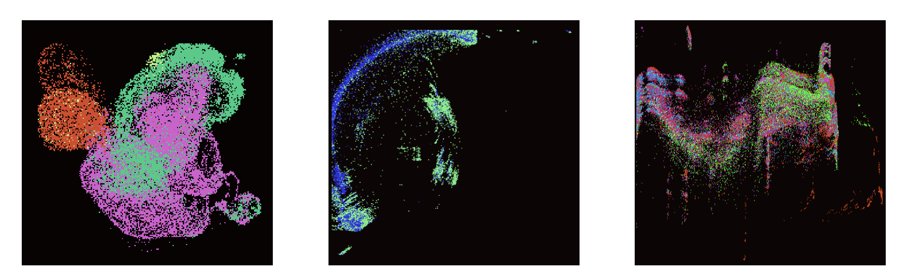
The Uniform Manifold Approximation and Projection (UMAP) methodology for Dimension Reduction can be used both as a general dimension reduction tool and as an interpretability/visualization tool, and here we use it for both. UMAP assumes data lies on a manifold and utilizes local approximations (k-nearest neighbor graphs) to represent the data’s topological and metric structure. Each local neighborhood is encoded as a fuzzy simplicial set, and then merged probabilistically to form a global topological structure (McInnes et al., 2020). Figure 10 provides a couple of examples of embeddings from different models and geospatial datasets projected into a lower-dimension feature space using UMAP, and overlaid with each sample’s target or label value.

UMAP scatter plots of embeddings for datasets with 4, 2, and 7 classes

UMAP scatter plots of embeddings for datasets with 4, 2, and 7 classes
Figure 10. Embeddings from different models and geospatial datasets with 4 classes (left), 2 classes (center), and 7 classes (right) projected into a 2D feature space using UMAP.


Notice that the separation of label sets in the projections degrades from left to right, indicating that the models increasingly struggle to represent class distinctions in a way that is easily recoverable in a low-dimensional space. This does not always mean that a model is fundamentally unable to represent the underlying data structure; in some cases, the representation may be more complex and non-linear, which makes faithful projection into two dimensions difficult. That limitation is important to keep in mind when interpreting these plots, but the analysis remains useful in many ways. The primary two points of utility in this context are described below.

First, complex representations leading to poor or muddled separation in the UMAP-projected space often signal that downstream learning tasks will be more challenging. A decoder trained on such embeddings must work harder to tease apart classes, may require more capacity or careful regularization, and can be more sensitive to hyperparameters and data preprocessing. Conversely, when classes form clean, well-separated clusters in these projections, it suggests that relatively simple decoders may be sufficient, which can guide architectural and training choices.

Second, these projections provide a bridge between model behavior and human interpretability. In scientific applications, our aim is not only to achieve high predictive performance but also to understand why a model behaves the way it does and how its representations relate to known processes. Visualizing how embeddings cluster, or fail to cluster, by class, region, or other attributes allows domain experts to assess whether a model organizes information in scientifically meaningful ways, to spot systematic confusions, and to generate new hypotheses. In that sense, manifold projections are both a diagnostic tool for model selection and a vehicle for scientific insight, which we view as essential for data science and deep learning applications in these domains.

Some additional limitations include:

  1. the use of stochastic operations leading to different runs or subsampling yielding varied results, and
  2. the quality and nature of these products are sensitive to hyperparameters. However, empirically, the authors note that while this is true, a general similarity of structure can be achieved relative to class separation if the representations of N classes are distinct enough.

While useful, the uncertainties of these tools require us to use multiple approaches to get a more comprehensive look at the state of model representation. To complement these qualitative projections, we next turn to data-kernel-based methods that quantify representational differences between encoders in a more statistically rigorous way.

Data Kernels for Inter-Model Embedding Comparisons

Encoder projections and embedding geometries are not directly comparable due to inherent incongruities, namely, differences in the dimensionality of original encodings or in their basis vectors. To address these discrepancies, we leverage recent advances in embedding space analysis and graph projection techniques, enabling the joint projection of transformations from diverse encoder architectures (Duderstadt et al., 2023). This encoding-centric analysis facilitates direct comparison of entire embedding spaces generated by different models.

Such an approach is especially valuable when downselecting from a large pool of candidate encoders. By quantifying representational similarity, we avoid exhaustive testing: models with highly similar encoding geometries are likely to yield comparable performance on a target task, meaning only representative models from each group need to be evaluated. Likewise, this methodology aids in constructing a taxonomy of applicable models tailored to specific tasks or domains.

Within a joint projection, each data point is represented N times, where N is the number of models under consideration. To assess the significance of differences between two representations of the same datum, we model the p-value distribution of representation distances, drawing on theoretical foundations from random graph literature. For a single model, resampling (via perturbation and bootstrapping) yields a rejection radius: a threshold delineating typical within-model embedding variation. When the paired representation of a sample from a different model falls outside of this radius, it indicates a materially different encoding of that sample. The probability of rejection tends to correlate with discrepancies in encoder training data and significant representational differences.

Finally, this technique can be iteratively applied: by generating a distance matrix that quantifies distances between N projections of identical samples across all embedding sets, and then applying dimensionality reduction again on the distance matrix, we obtain a streamlined, task-relevant comparison of model representations via a single point representative of each embedding set/model representation.

Like performance metrics for downstream tasks, each of these methodologies provides a piece of the full picture, and collectively they can provide a more comprehensive view of a model’s representational skill and potential generalizability.

Section B: The Framework

Link to original repository

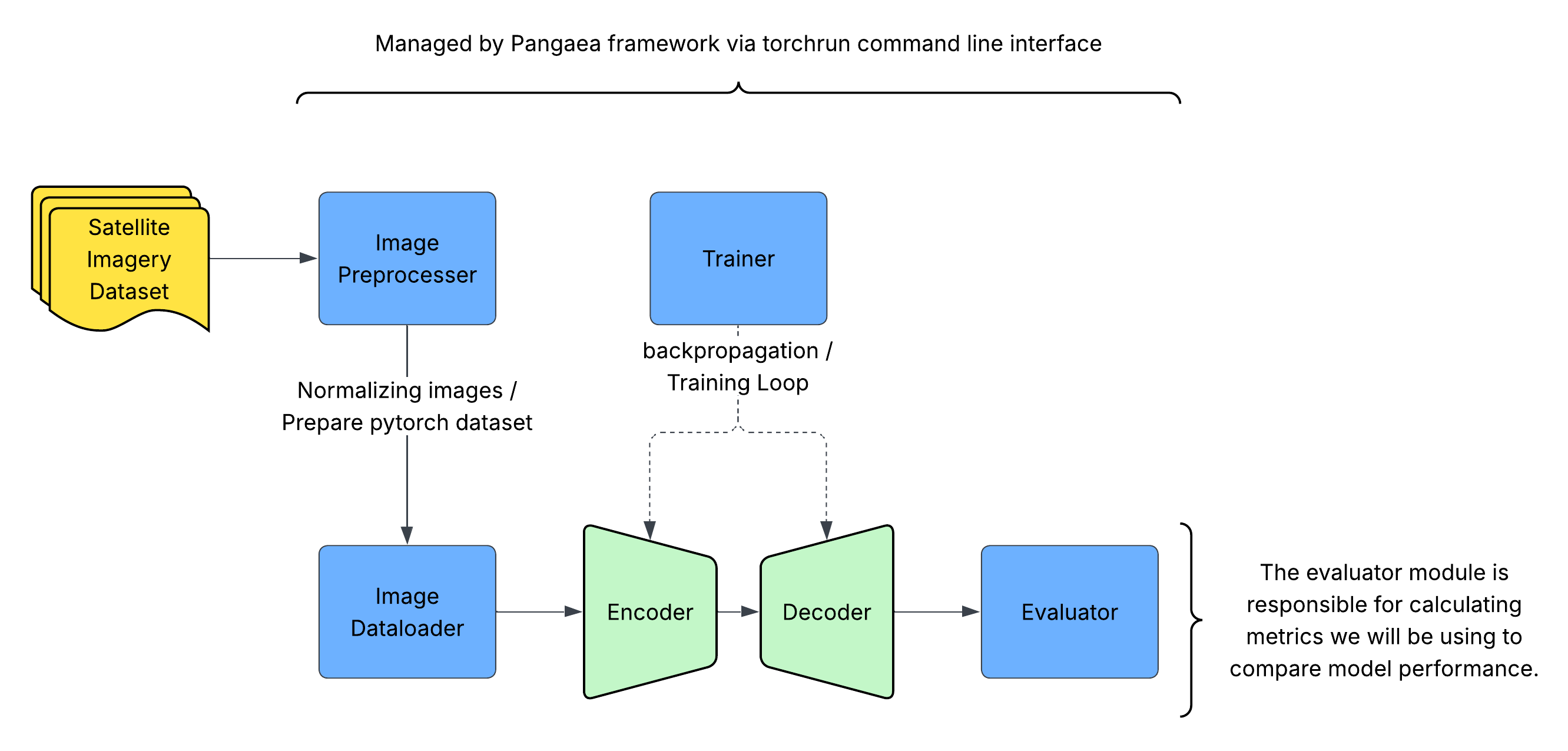
We apply the Pangaea Bench benchmarking framework originally developed by the ESA Phi Lab team (Marsocci et al., 2024). While other teams are developing frameworks, Pangaea conveniently integrates many of the more popular remote sensing foundation models into its pure PyTorch framework, along with several well-established benchmarking datasets. Figure 11 shows the design of the Pangaea framework. It also includes a relatively simple dataset integration scheme along with additional decoder heads and encoder evaluation methodologies integrated by the team at Spatial Informatics Group. The limited dependency list is especially beneficial for small-scale demonstrations such as this learning notebook. You will find similar themes to those found in previous chapters of the Applied Deep Learning Book, such as dataloaders, PyTorch modules, loss functions, etc. These are not exclusive to training end-to-end models, and in fact, the workflow is almost the same! The EOFMs are intended to solve the same segmentation, classification, or regression problems differently. Here, we focus on the additional considerations that come with using an EOFM for segmentation.

Diagram of the Pangaea-Bench benchmarking framework structure

Diagram of the Pangaea-Bench benchmarking framework structure
Figure 11. Diagram of Pangaea’s general structure.


The ‘torchrun’ Command

The torchrun command is a utility provided by PyTorch to launch distributed training jobs across multiple processes, nodes, or GPUs See torchrun documentation on environment variables for more details. It replaces the older torch.distributed.launch and is part of the torch distributed module. torchrun is designed to be simple and flexible, making it easier to scale up training scripts with minimal changes. At its core, torchrun sets up the environment variables necessary for distributed training, such as RANK, WORLD_SIZE, and MASTER_ADDR, and then spawns multiple processes, one per GPU or per node, depending on the configuration. This enables parallel training using frameworks like DistributedDataParallel (DDP), which helps synchronize gradients and significantly reduce training time. This will be especially useful for training larger networks; however, for this demonstration, we will only use it to run on a single machine.

The Pangaea benchmarking framework is a lightweight wrapper around this command to handle most of the boilerplate code that comes with training a neural network. This includes establishing the training loop, calculating metrics, logging, and the datasets/dataloaders associated with the benchmarks. Several command options are available and can be found in ./pangaea-bench/configs. We only use the subset exemplified below in this demonstration notebook, but many more are available. Config files for the dataset, decoder, and encoder are associated with a PyTorch module that the framework instantiates based on the configurations provided.

!torchrun pangaea-bench/pangaea/run.py \                                ##### The torchrun entry command
    --config-name=train \                                               ##### configuration name which can be found in ./pangaea-bench/configs
    work_dir=checkpoints \                                              ##### the directory relative to the working directory to store checkpoint outputs
    dataset=mtbs \                                              ##### the dataset config file found in ./pangaea-bench/configs
    encoder=dofa\                                                       ##### the encoder config file found in ./pangaea-bench/configs
    decoder=seg_fcn\                                                    ##### the decoder config file found in ./pangaea-bench/configs
    preprocessing=seg_default\                                          ##### preprocessing steps associated with the task type (e.g normalizing images)
    criterion=cross_entropy \                                           ##### the loss function on which to optimize the training cycle
    task=segmentation \                                                 ##### task type (others include classification and regression)
    use_wandb=true \                                                    ##### whether to use the online logging software
    task.trainer.n_epochs=16 \                                          ##### number of epochs to limit training
    task.trainer.log_interval=1 \                                       ##### logging interval of calculated metrics
    task.trainer.ckpt_interval=16 \                                     ##### how often to save checkpoints based on metrics
    encoder.encoder_weights=pretrained_models/DOFA_ViT_base_e100.pth    ##### path to pretrained weights of the FM

Section C: Encoder Assessments

Frozen vs Unfrozen vs Random vs LoRA

Testing frozen, unfrozen, and randomly initialized pretrained encoders is useful in understanding the value and applicability of transfer learning for a specific task. A frozen encoder uses pretrained weights without updating them during training (Marsocci et al., 2024). This setup helps evaluate how useful the pretrained features are on their own, especially in cases where the target dataset is small or the model is prone to overfitting. In contrast, an unfrozen encoder allows those pretrained weights to be updated, enabling the model to adapt its learned representations to suit the target task better. This approach often yields better performance when sufficient labeled data is available, and the task deviates from the original pretraining domain; however, it requires additional gradients to be computed and stored. On the other hand, a randomly initialized encoder serves as a baseline, providing a measure of how well the model performs without any prior knowledge. Comparing results from this setup against those using pretrained weights helps quantify the benefits of pretraining in terms of training time and overall final performance. It’s worth noting that depending on the task and the amount of available training data, the randomly initialized encoder may never achieve the same results as an unfrozen pretrained model. This behavior is still an ongoing area of research.

Overall, these three basic configurations allow for a comprehensive assessment of whether transfer learning is useful, whether fine-tuning improves results, and whether pretraining is necessary at all for a specific task. There is a fourth method, which we will not use here, called Low Rank Adaptation (LoRA), and is somewhat of a compromise between a fully frozen and unfrozen encoder (Hu et al., 2021). LoRA is a technique used to efficiently fine-tune large pretrained neural networks by injecting small, trainable weight matrices into the model, while keeping the original weights frozen. This is typically reserved for larger models (i.e greater than 300m parameters). Traditional fine-tuning updates all parameters of a model, which becomes expensive for large models. LoRA avoids this by approximating the weight updates as the product of two low-rank matrices, significantly reducing the number of trainable parameters. This low-rank decomposition acts as a bottleneck, enforcing efficiency and reducing overfitting. LoRA has gained popularity particularly with large language models. It also enables modular fine-tuning where separate LoRA modules can be swapped in for different tasks, making it attractive for applications requiring task specialization without retraining the entire model.

Highlighted Models

For the encoder evaluation, we will take a look at a large set of pretrained encoders available within Pangaea-Bench. From there, we will focus fine-tuning on a single task for 3 frozen encoder variations: Dynamic One-For-All (DOFA), Contrastive Radar-Optical Masked Autoencoder (CROMA), and Prithvi 1.0 (described below). Below is a brief introduction to the models we will focus on in the fine-tuning process and beyond. #### DOFA

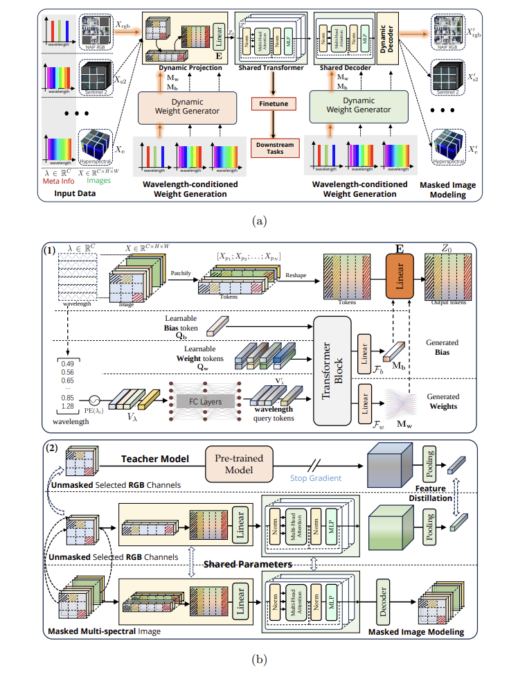
DOFA is a transformer-based model (Figure 12a) that is optimized on both a mask image modeling objective and a self-distillation objective (Figure 12b). DOFA’s major contribution is its wavelength-conditioned dynamic patch embedding, in which the central wavelength of a given sensor is used to derive the weights for processing the respective data (Xiong et al., 2024). It is apparent from this that the model developers’ approach is targeting flexibility and generalizability across multiple modalities and does so fairly well. And yet, there are still open questions. For example, wavelength and reflectance do not necessarily translate to amplitude data from SAR; does this matter? Benchmarking metrics will tell you no, but do keep in mind the underlying reasons for these behaviors.

DOFA architecture diagram showing dynamic patch embedding and weight generator

DOFA architecture diagram showing dynamic patch embedding and weight generator
Figure 12: (a) Architecture design. DOFA builds on masked image modeling by processing input images with any number of channels within a single framework. (b) Dynamic weight generator and continual training framework from (Xiong et al., 2024).

Prithvi 1.0

Prithvi v1.0 is one of the earliest foundation models and the simplest of the three models tested in this demonstration (Jakubik et al., 2023). Developed by the NASA IMPACT team, Prithvi v1.0 (Figure 13) is a masked autoencoder trained exclusively on Harmonized Landsat and Sentinel (HLS) data, with an added module for handling spatial and temporal context. The Prithvi model’s training on HLS data provides an interesting opportunity for discussion in our benchmarking: do we expect a model pretrained on HLS data to perform best on tasks using similar HLS imagery? Equally, to what extent do we expect models to adapt to similar but distinct modalities? Especially those which overlap, such as Sentinel-2 and non-harmonized Landsat. As with other models described in this chapter, the Prithvi team is actively working to improve their model and has released new versions of their architecture and model weights. If the reader is interested, we recommend working towards reproducing the results of these experiments, with Prithvi v2.0 (Szwarcman et al., 2025).

Prithvi masked autoencoder pretraining architecture diagram

Prithvi masked autoencoder pretraining architecture diagram
Figure 13: Masked autoencoder diagram for Prithvi’s pretraining from (Jakubik et al., 2023).

CROMA

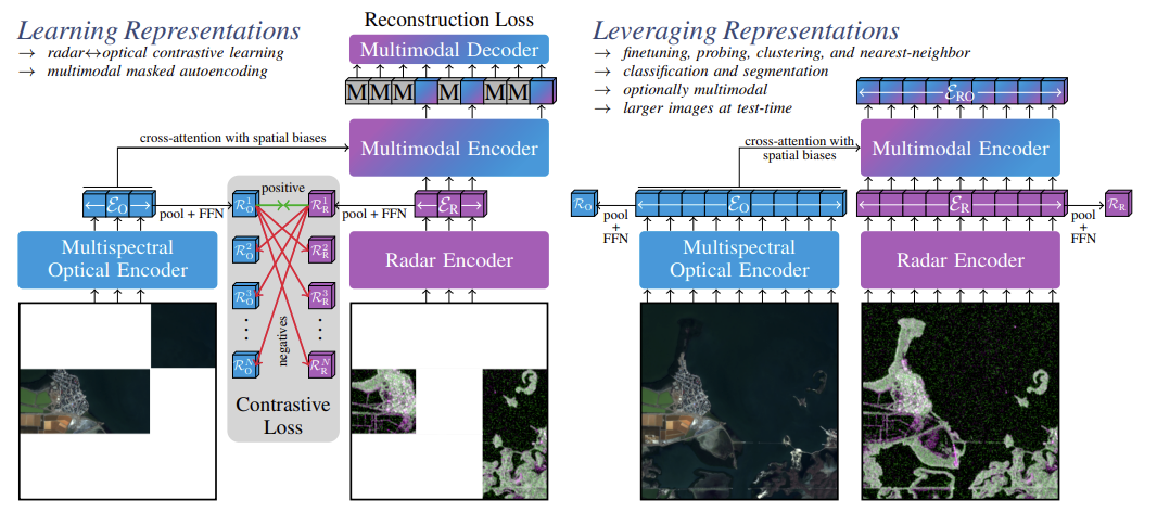
CROMA (Figure 14) is another transformer-based model whose pretraining approach combines both MIM and contrastive learning (Fuller et al., 2023). Rather than contrasting positive and negative samples, the CROMA framework contrasts optical and radar data using separate encoders, then combines those embeddings using cross-attention with an additional transformer encoder. The output of this joint encoder is then randomly masked and trained in a typical encoder-decoder MIM style. The optical encoder requires all 12 spectral bands from Sentinel 2, while the radar encoder requires the 2 polarization bands from Sentinel 1. In our downstream task, we are limited to 6 harmonized spectral bands. How can we expect this to impact our results?

CROMA pretraining framework and encoding workflow diagram

CROMA pretraining framework and encoding workflow diagram
Figure 14: (Left) Pretraining framework for CROMA. (Right) Encoding workflow for leveraging internal representations.

Encoder Weight-Matrix Analysis

Before we look at the encoders relative to the input data, let’s evaluate the weight matrices. For this analysis, the dataset information is only used to extract metadata information within the Pangaea library so that the results will be the same for hlsburnscars and mtbs configuration input values. Some of these models support multi-modal inputs, or inputs from different instrument types (i.e., optical, radar, etc.). When additional modalities are brought in, some models leverage additional layers or encoders altogether. Here, both test cases are using optical only, so it is not a concern.

Below are the example commands for CROMA, DOFA, and Prithvi. The commands for all other encoders can be found here: Multi-Encoder Per-Layer Weight Matrix Analysis

Show code
%%time

#Ensure we are in the correct directory
%pushd /content/pangaea-bench/pangaea/encoder_analysis/

!python3 weight_watcher.py dataset=mtbs encoder=croma_optical \
    preprocessing=seg_resize_input_layer task=segmentation

#Move output to location for longer-term storage
!mv img/* ww/croma/
!mv ww-img/* ww/croma/

!python3 weight_watcher.py dataset=mtbs encoder=dofa \
    preprocessing=seg_resize_input_layer task=segmentation

#Move output to location for longer-term storage
!mv img/* ww/dofa/
!mv ww-img/* ww/dofa/

!python3 weight_watcher.py dataset=mtbs encoder=prithvi \
    preprocessing=seg_resize_input_layer task=segmentation

#Move output to location for longer-term storage
!mv img/* ww/prithvi/
!mv ww-img/* ww/prithvi/

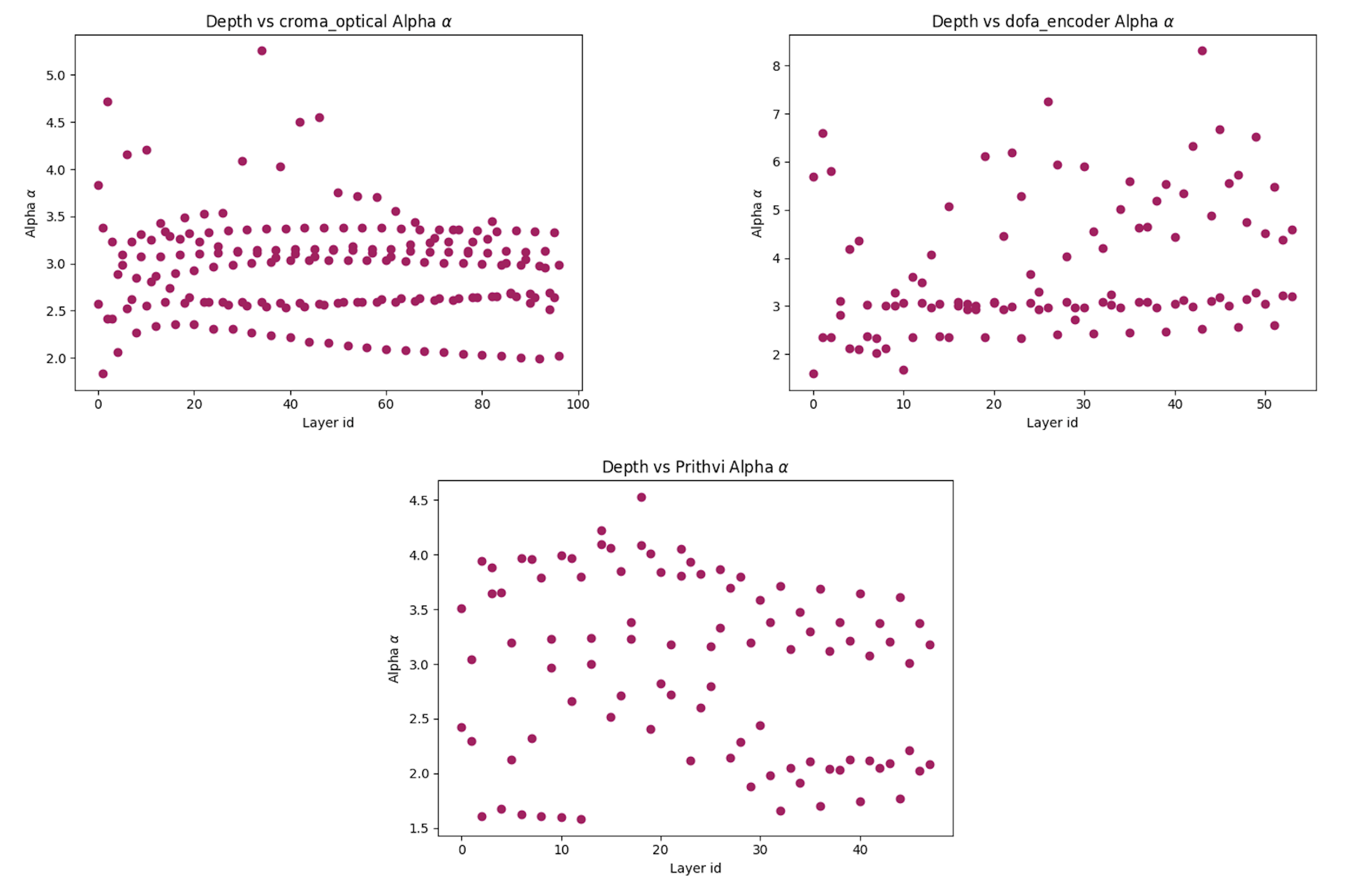
Additional details are produced in plots generated by the commands run, but we will use the per-layer \(\alpha\) plots in Figure 15 to provide a top-level summary of the findings. These plots summarize each layer’s empirical spectral density using the power-law exponent \(\alpha\); Lower \(\alpha\) values indicate heavier tails and potential overfitting, whereas higher \(\alpha\) values suggest lighter tails and possible underfitting. . CROMA appears to have the most consistently well-trained layers, with most \(\alpha\) values staying within the desired [2,5] range, and deviations outside this range being very minimal. Prithvi appears to have a handful of layers that are overfit to a small degree, and DOFA has a somewhat evenly distributed set of layers throughout the model that appear to be underfit.

There are a few layers that deviate below 2 at the beginning of each model, which is a pattern identified in previous studies of vision models using the weight watcher tool. The current hypothesis is that most high-level features learned in early layers of vision models are similar across all scenes in a large training set, so the early layers in a model, typically the ones that learn these high-level features, tend toward overfitting/a lack of generalizability. Here, the deviations only appear to be minor.

Alpha parameter versus layer depth plots for CROMA, Prithvi, and DOFA

Alpha parameter versus layer depth plots for CROMA, Prithvi, and DOFA
Figure 15. Plots containing the \(\alpha\) summary parameter from the model weight matrix analysis done for CROMA (top left), Prithvi (bottom center), and DOFA (top right).


This analysis not only informs us about performance considerations when using these models with frozen weights, but can also provide insight into what we need to take into account if we are to fine-tune all or a subset of the weights of these encoders. For example:

1) Which models’ overfit layers might be more prone to a phenomenon called catastrophic forgetting, where performance significantly dips after fine-tuning due to the information gained in pretraining being lost or overwritten?

2) Which model’s layers may need more time to learn/optimize during the fine-tuning phase, due to being underfit in pretraining?

Resource Requirements - FLOPS, MACS, and Parameter Counts

Next, we will look at the computational and storage requirements for each model. Spectral analysis tells us something about how encoders use their parameters; we also need to know how many parameters and how much compute they require in the first place.

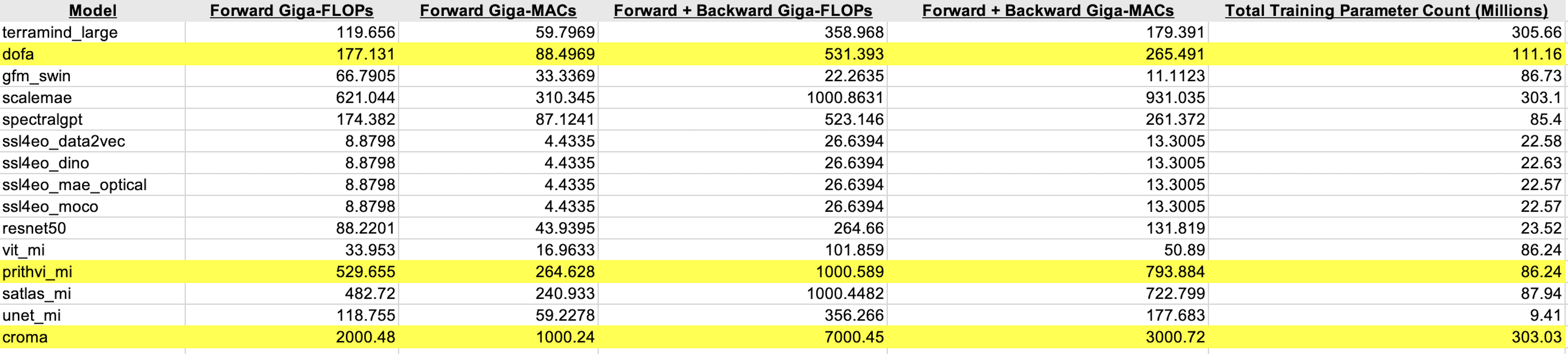
Below are the example commands for CROMA, DOFA, and Prithvi. The commands for all other encoders can be found here: MTBS Multi-Encoder Resource Consumption Estimation. Table 1 provides the results of the computation for a larger set of models supported by Pangaea, with the models in focus highlighted. The authors feel it is important to put these comparisons into a wider context to understand resource requirements relative to a wider set of models being used in the field. For additional information on the wider set of models, see (Marsocci et al., 2024) and the papers referenced within it.

Here we use a small amount of data to pass into the resource utilization profiler, but since we are looking at inference performance over a single sample, relative resource usage does not change across the two datasets in use here, and there are only minor shifts in the results. Therefore, we only look at output generated using the MTBS data here. In subsequent steps, we will look at both separately. As with the weight-matrix analysis, if other modalities are being used, the resource consumption outputs will likely change.

Show code
%%time

import os
os.environ['PYTHONPATH'] += ":/content/calculate-flops.pytorch/"

#Ensure we are in the correct directory
%pushd /content/pangaea-bench/pangaea/encoder_analysis/

!python3 compute_flops.py dataset=mtbs   encoder=croma_optical  preprocessing=seg_irregular_images    task=segmentation
!python3 compute_flops.py dataset=mtbs   encoder=dofa  preprocessing=seg_irregular_images    task=segmentation
!python3 compute_flops.py dataset=mtbs   encoder=prithvi  preprocessing=seg_irregular_images    task=segmentation

Table comparing resource consumption of CROMA, DOFA, and Prithvi models

Table comparing resource consumption of CROMA, DOFA, and Prithvi models
Table 1. Resource consumption of the three encoders relative to common pretrained and randomly initialized models. Note the diversity in the amount of calculations required by the different models. We will touch on this in the following section.


Here we can see that CROMA, DOFA, and Prithvi stand out as some of the largest models, with the number of operations for forward and backward passes also in the higher range across the set. These models are being used here to provide an example and do not necessarily outperform all others when compared to every other permutation possible within Pangaea and those without. The authors re-emphasize that the smallest and most optimized (least resource-intensive) model that provides a good representation of the features of interest in the dataset and a good enough (typically task-dependent) performance on the ultimate task should be chosen.

Embedding generation

Next, we will take the input dataset and pass it through the pretrained encoders to get model-specific representations, or embeddings, for each input scene. Below are example commands for the CROMA, DOFA, and Prithvi encoders and both the MTBS and HLS Burn Scars datasets. We also generate these for 16 other encoders for both cases (pretrained and randomly initialized where available). Again, while we do not go into detail on the full set of models here, the authors find it important to do these inter-comparisons within a wider array of model choices.

Additional example commands can be found here: MTBS Multi-Encoder Embedding Generation Script and HLS Multi-Encoder Embedding Generation Script

Show code
%%time

#Ensure we are in the correct directory
%pushd /content/pangaea-bench/pangaea/encoder_analysis/

#!python3 embed.py dataset=hlsburnscars encoder=croma_optical preprocessing=seg_irregular_images task=segmentation
!python3 embed.py dataset=mtbs encoder=croma_optical preprocessing=seg_irregular_images task=segmentation

#!python3 embed.py dataset=hlsburnscars encoder=dofa preprocessing=seg_irregular_images task=segmentation
!python3 embed.py dataset=mtbs encoder=dofa preprocessing=seg_irregular_images task=segmentation

#!python3 embed.py dataset=hlsburnscars encoder=prithvi preprocessing=seg_irregular_images task=segmentation
!python3 embed.py dataset=mtbs encoder=prithvi preprocessing=seg_irregular_images task=segmentation

UMAP Projection and KNN Graph Generation

Now that we have the embeddings, we can project them onto a lower-dimensional manifold and generate a KNN-Graph from that representation. Below are example commands for CROMA, DOFA, and Prithvi. The commands for all other encoders can be found here: MTBS Multi-Encoder UMAP Projection and KNN-Graph Generation and HLS Burn Scars Multi-Encoder UMAP Projection and KNN-Graph Generation

Show code
%%time

#Ensure we are in the correct directory
%pushd /content/pangaea-bench/pangaea/encoder_analysis/

!python3 knn_graph_gen.py dataset=hlsburnscars \
                          encoder=croma_optical \
                          preprocessing=seg_irregular_images \
                          criterion=cross_entropy \
                          task=segmentation

!python3 knn_graph_gen.py dataset=hlsburnscars \
                          encoder=dofa \
                          preprocessing=seg_irregular_images \
                          criterion=cross_entropy \
                          task=segmentation

!python3 knn_graph_gen.py dataset=hlsburnscars \
                          encoder=prithvi \
                          preprocessing=seg_irregular_images \
                          criterion=cross_entropy \
                          task=segmentatio

!python3 knn_graph_gen.py dataset=mtbs \
                          encoder=croma_optical \
                          preprocessing=seg_irregular_images \
                          criterion=cross_entropy \
                         task=segmentation

!python3 knn_graph_gen.py dataset=mtbs \
                          encoder=dofa \
                          preprocessing=seg_irregular_images \
                          criterion=cross_entropy \
                          task=segmentation

!python3 knn_graph_gen.py dataset=mtbs \
                          encoder=prithvi \
                          preprocessing=seg_irregular_images \
                          criterion=cross_entropy \
                          task=segmentation

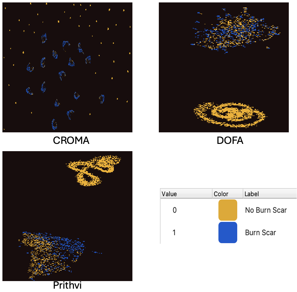
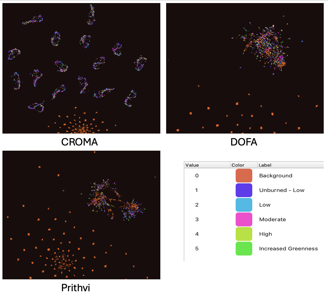
We can use these plots first to do a qualitative analysis if we compare these UMAP plots to those in Figures 16 and 17, where we can see weak to moderate separations of the classes for all models and can take away the fact that these are not an easy task for these models out of the box.

UMAP Analysis HLS Burn Scars

UMAP embedding plots for CROMA, DOFA, and Prithvi on HLS Burn Scars data

UMAP embedding plots for CROMA, DOFA, and Prithvi on HLS Burn Scars data
Figure 16. A plot of the embeddings generated from CROMA (top left), Dofa (top right), and Prithvi (bottom left) for samples from the test split of the HLS Burn Scars dataset projected onto a low-dimensional (2D) manifold via UMAP and overlaid with their associated target value. The key for the targets is on the bottom right.


In all three cases, to varying degrees, there is an intermixing of the label values. CROMA appears to do the best at separating subsets of the classes in different ways, and Prithvi does keep some distinction between them. In contrast, DOFA appears to have the hardest time representing the classes distinctly in its embedding space, as demonstrated by a lack of clear separation of the positive label from the negative one anywhere in the plot. Some of the background pixels are clearly separated from the rest of the samples in each case, but there remains a significant amount of class mixing in the remainder of the plots.

UMAP Analysis MTBS

UMAP embedding plots for CROMA, DOFA, and Prithvi on the MTBS dataset

UMAP embedding plots for CROMA, DOFA, and Prithvi on the MTBS dataset
Figure 17. A plot of the embeddings generated from CROMA (left), DOFA (center), and Prithvi (right) for samples from the test split of the MTBS dataset projected onto a low-dimensional (2D) manifold via UMAP and overlaid with their associated target value. The key for the targets is on the bottom right.


Again, but at a higher rate than in the HLS Burn Scars plots, there is an intermixing of the label values. All of the models appear to have a difficult time discerning among the classes, beyond separating some of the background class from the rest of the samples.

As mentioned before, this methodology is not perfect, and we are removing representative information from embedded samples by reducing the feature space. However, trade-offs must be made for interpretability and analysis of model performance because results need to be human-interpretable to be useful. If a model is more easily able to represent distinctions between samples in a simplified way at a higher dimension, those distinctions will likely be picked up in this lower-dimensional space.

Inter-Model Embedding Comparisons Using Data Kernels

Here, we take the previously generated KNN graphs and use a data-kernel-based projection to project all embedding samples into a uniform feature space for subsequent analysis. Below are the example commands for CROMA, DOFA, and Prithvi. The commands for all other encoders can be found here: MTBS Multi-Encoder Embedding Comparison and HLS Burn Scars Multi-Encoder Embedding Comparison

Show code
%%time

#Ensure we are in the correct directory
%pushd /content/pangaea-bench/pangaea/encoder_analysis/

#!python3 data_kernel_analysis.py dataset=hlsburnscars   task=segmentation
!python3 data_kernel_analysis.py dataset=mtbs   task=segmentation

For both datasets, we start by generating a scatter plot of all samples to visualize similarities and differences (Figures 18 and 22). Next, we reduce the dimensionality again, creating a manifold where each set of embeddings is represented by a single point (Figures 19 and 23). With joint projections from paired models, we can model the p-value distribution, given the null hypothesis based on sample distance representations using ideas drawn from random graph theory to define this baseline. In other words, paired data that falls outside of a rejection radius is represented significantly differently.

Statistical tests between these representations provide insight into knowledge gaps unique to each model, highlighting differences in what they have learned or failed to capture as a result of their training regime or data selection process. These tests suggest that, although foundation models are individually designed to serve as unifying generalist tools, the representations they learn remain distinct from one another.

Embedding Space Comparisons - HLS Burn Scars

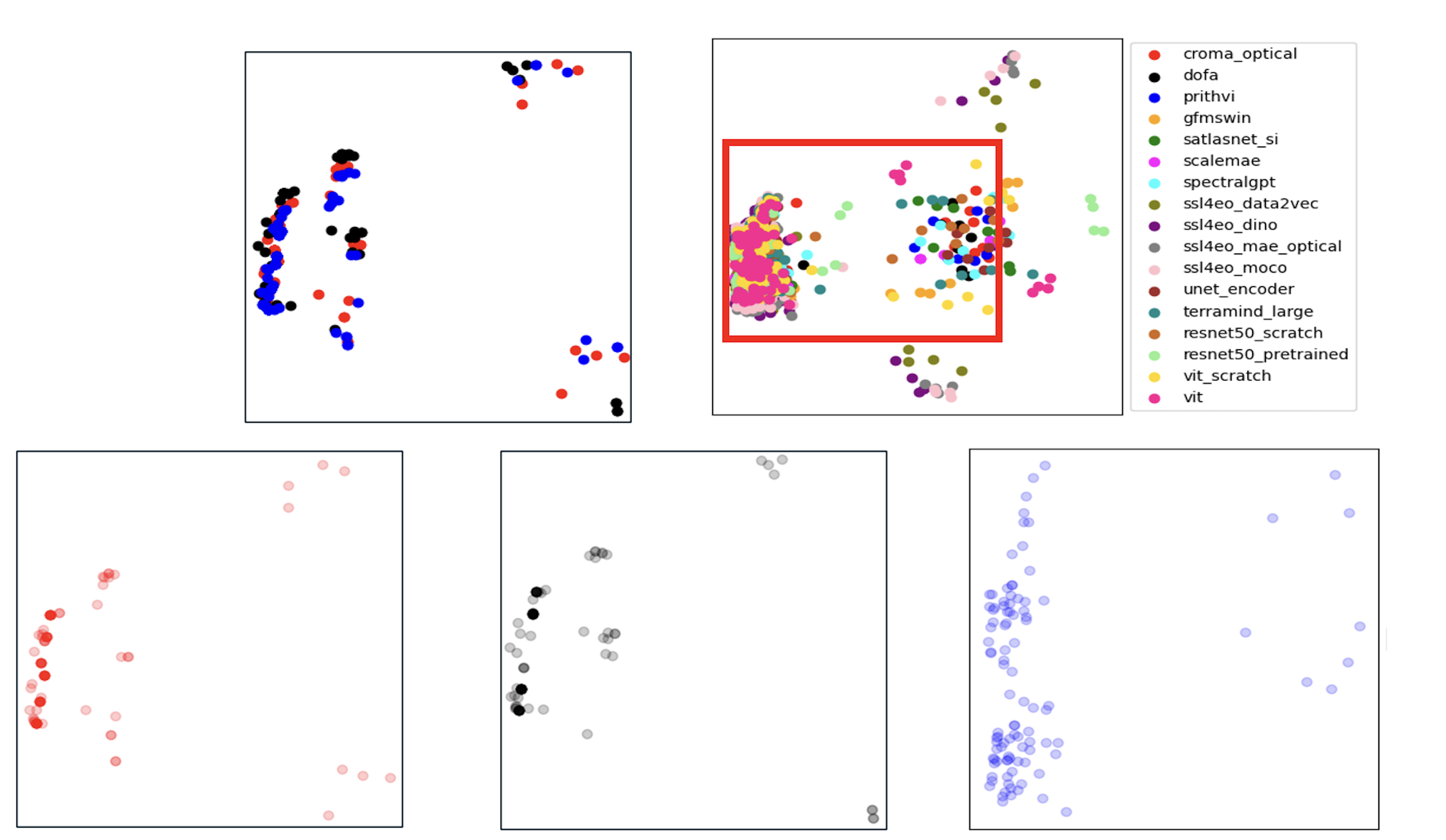
Figure 18 provides sample-wise scatter plots for a subset of samples projected into the uniform collective embedding space. This is shown for the models in focus (top left), a larger set of models supported by Pangaea-Bench (top right), as well as individual plots for each model in focus, with an additional visualization of spatial density (bottom), which will come in handy in this analysis.

Scatter plots of joint embedding projections for HLS Burn Scars across models

Scatter plots of joint embedding projections for HLS Burn Scars across models
Figure 18. A depiction of the joint embedding projection for the embeddings of a subset of the HLS Burn Scar data for the three models of focus here (top left) as well as a larger set of models supported by Pangaea-Bench (top right). The bottom row depicts a zoom-in of CROMA’s (left), DOFA’s (center), and Prithvi’s (right) samples in the embedding space, with opacity used to represent the spatial density of samples. The red box in the top-right figure indicates the subsetted area in the full embedding where these models have samples projected. The plots in the top-left and bottom rows contain only this subset area.


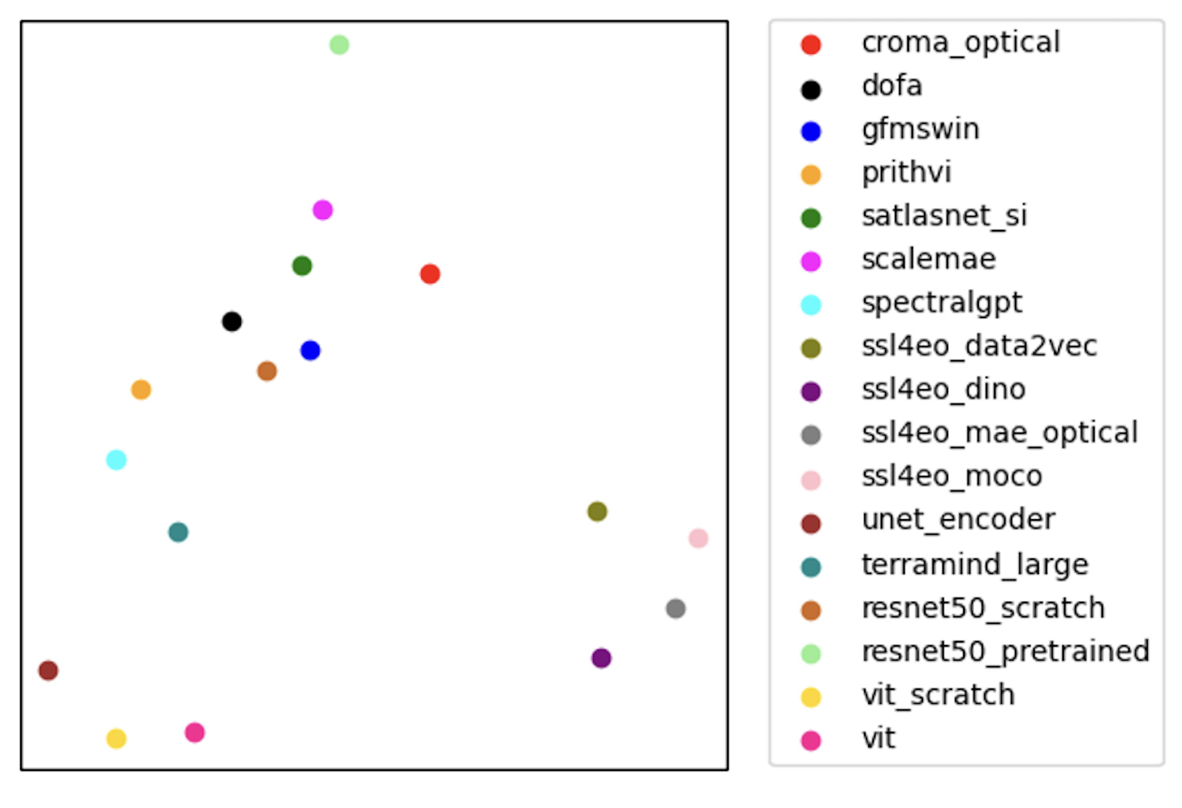
In Figure 19, we can see that DOFA and Prithvi are relatively close together, although it does not appear that they belong to a distinct single cluster of models.

Distance matrix plot of collapsed embedding spaces for HLS models

Distance matrix plot of collapsed embedding spaces for HLS models
Figure 19. A depiction of collapsing the embedding spaces into single points to visualize and measure population-level representational differences.


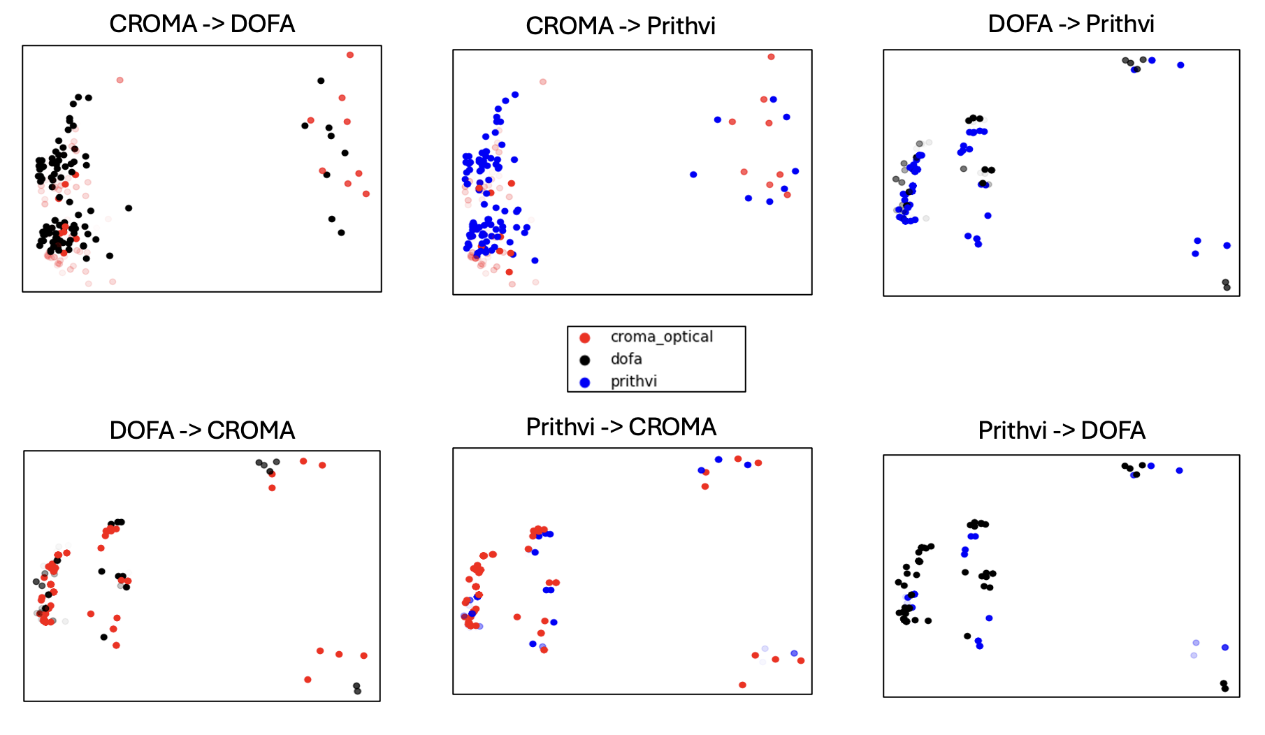
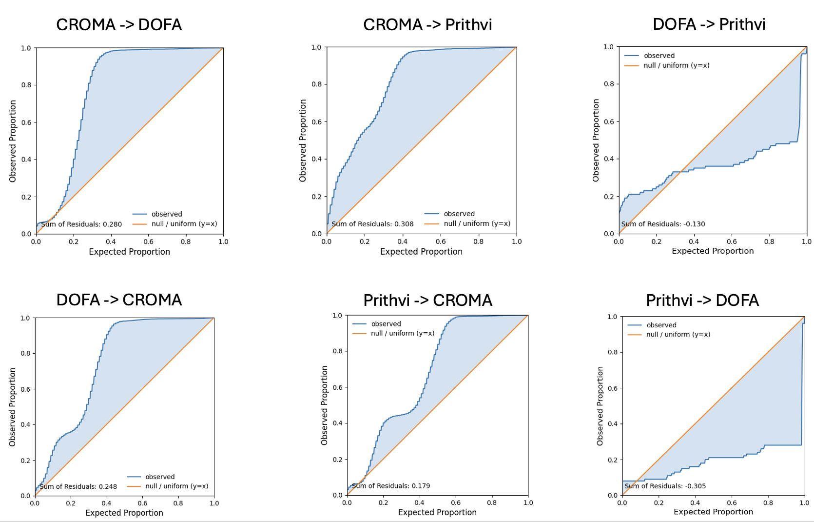
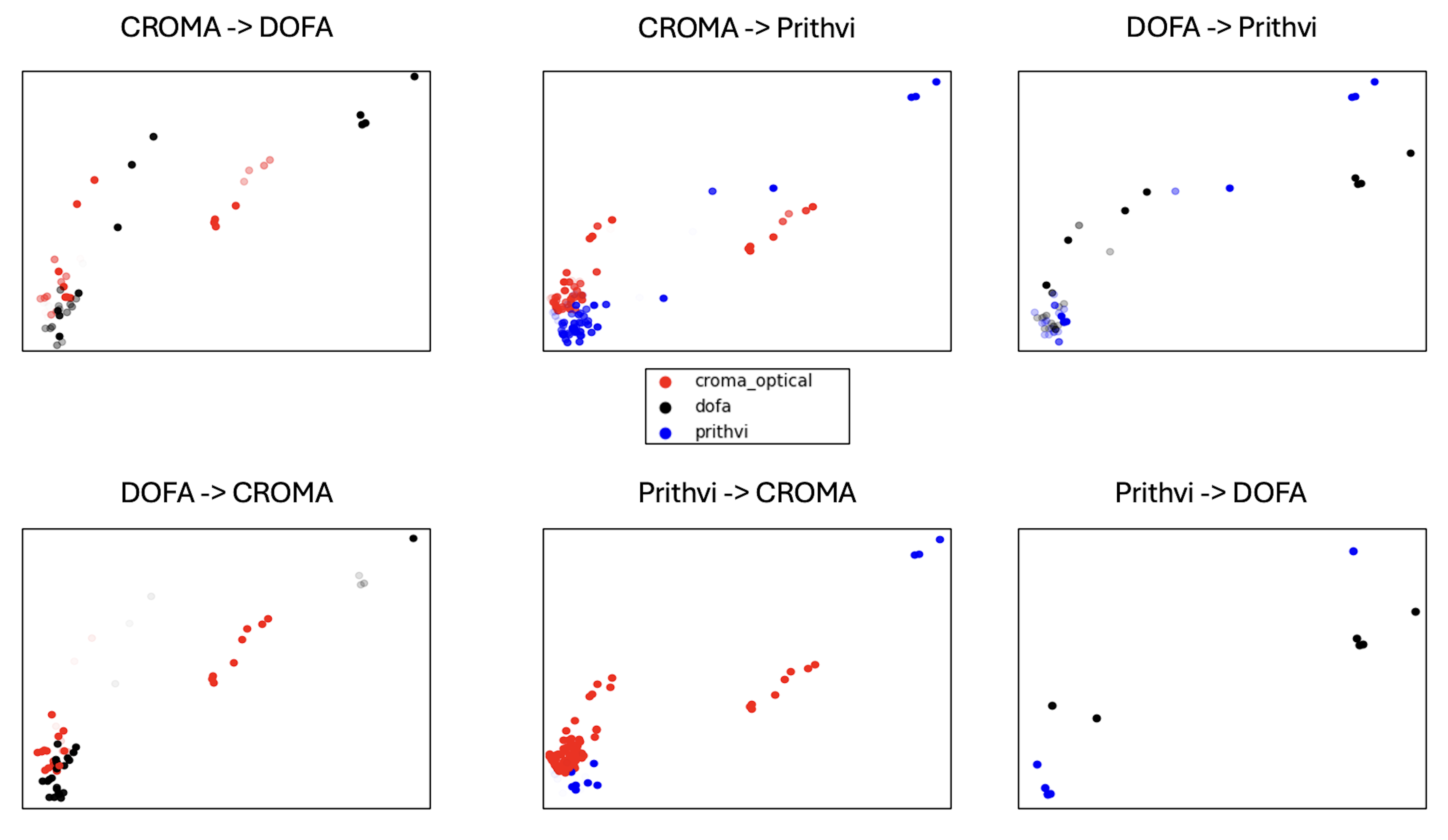
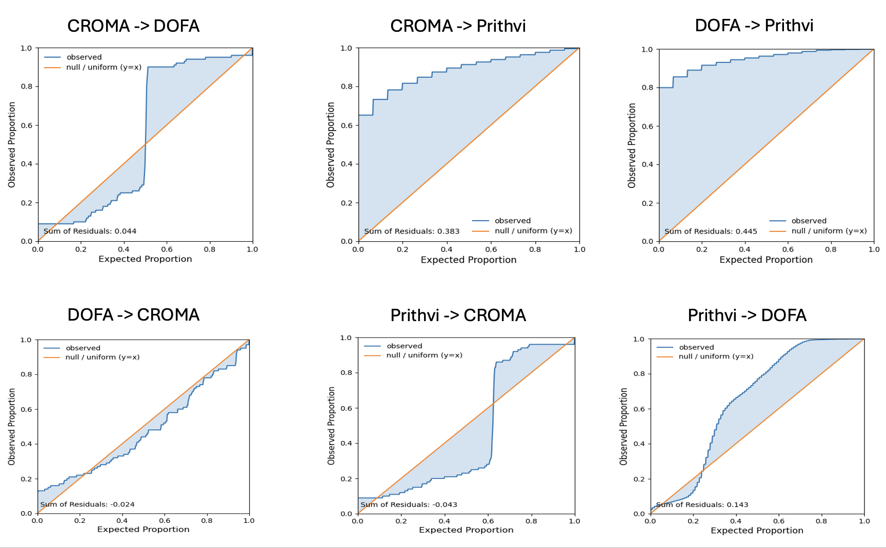
Figures 20 and 21 show pairwise comparison plots and the pairwise p-value distributions of differences between the two representations of the same samples, as described above. We can see that the representations are somewhat similar in the case of DOFA vs Prithvi, but otherwise clearly not the same. This is demonstrated by the number of samples with small p-values (less opaque samples in Figure 20) as well as p-value distribution plots in Figure 21. The p-value distributions in the comparisons of CROMA vs DOFA and CROMA vs Prithvi indicate strong dissimilarity, with heavy leftward shifts of the distribution (blue line) indicating rejection of the null hypothesis. In the case of DOFA vs Prithvi, the rightward shift indicates representational similarity.

Scatterplots comparing pairwise representational similarity between models using p-values, HLS data

Scatterplots comparing pairwise representational similarity between models using p-values, HLS data
Figure 20. Scatterplots of the embedding projections being used to measure population-level representational shifts between pairs of models. Here, the sample set from the model being compared against is plotted, and the model we are measuring deviation from has its samples overlaid on top. The opacity has an inverse relationship to the p-value of a given sample. All values with a p-value close to or equal to 1 are colored white here and therefore do not show up. Comparison datasets are on the left of the arrow and reference datasets are on the right for each plot title.


Distribution plots of p-values for each pair of models, HLS dataset

Distribution plots of p-values for each pair of models, HLS dataset
Figure 21. The distribution of p-values under the null hypothesis for each ordered pair of models. Comparison datasets are on the left of the arrow and reference datasets are on the right for each plot title.


The comparisons of Prithvi and CROMA samples (center top and bottom) as well as Prithvi and DOFA (right top and bottom) provide an interesting aside. Notice that when CROMA or DOFA embeddings are used as the comparison set and Prithvi as the reference (center top and right top), we get a lower measure of similarity in the set of plots compared to the plots generated when the roles of the datasets are swapped. This is due to differences in the spread of each model’s samples in the collective embedding space. The rejection radius for CROMA and DOFA is larger than for Prithvi. Thus, when we use CROMA or DOFA as reference, more sample tests accept the null hypothesis. We can see these patterns show up in the density-scaled scatter plots in Figure 18 as well as the inverse-p-value scaled ones in Figure 20. All of these analyses are consistent with the varying qualities observed in Figures 16 & 17.

Embedding Space Comparisons - MTBS

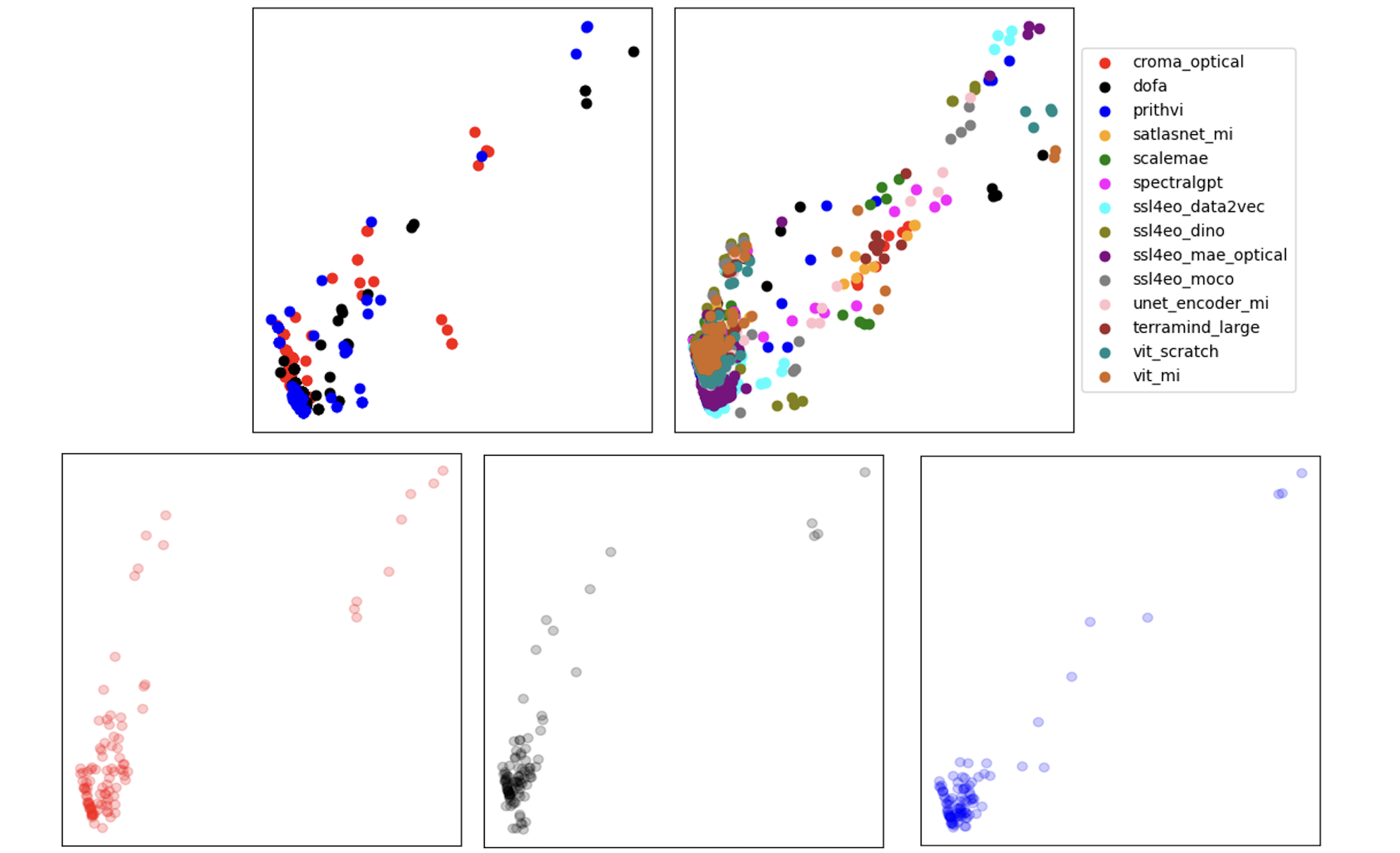
Figure 22 provides sample-wise scatter plots for a subset of samples projected into the uniform collective embedding space for the MTBS case. Because the reprojected embeddings for these models and this data span a wider set of the embedding field, we do not subsample for the 3-model and single-model scatterplots, as in Figure 18.

Scatter plots of joint embedding projections for the MTBS dataset across models

Scatter plots of joint embedding projections for the MTBS dataset across models
Figure 22. A depiction of the joint embedding projection for the embeddings of the MTBS dataset and the three models of focus here (top left) as well as a larger set of models supported by Pangaea-Bench (top right). The bottom row depicts CROMA’s (left), DOFA’s (center), and Prithvi’s (right) samples in the embedding space, with opacity used here to represent the spatial density of samples.


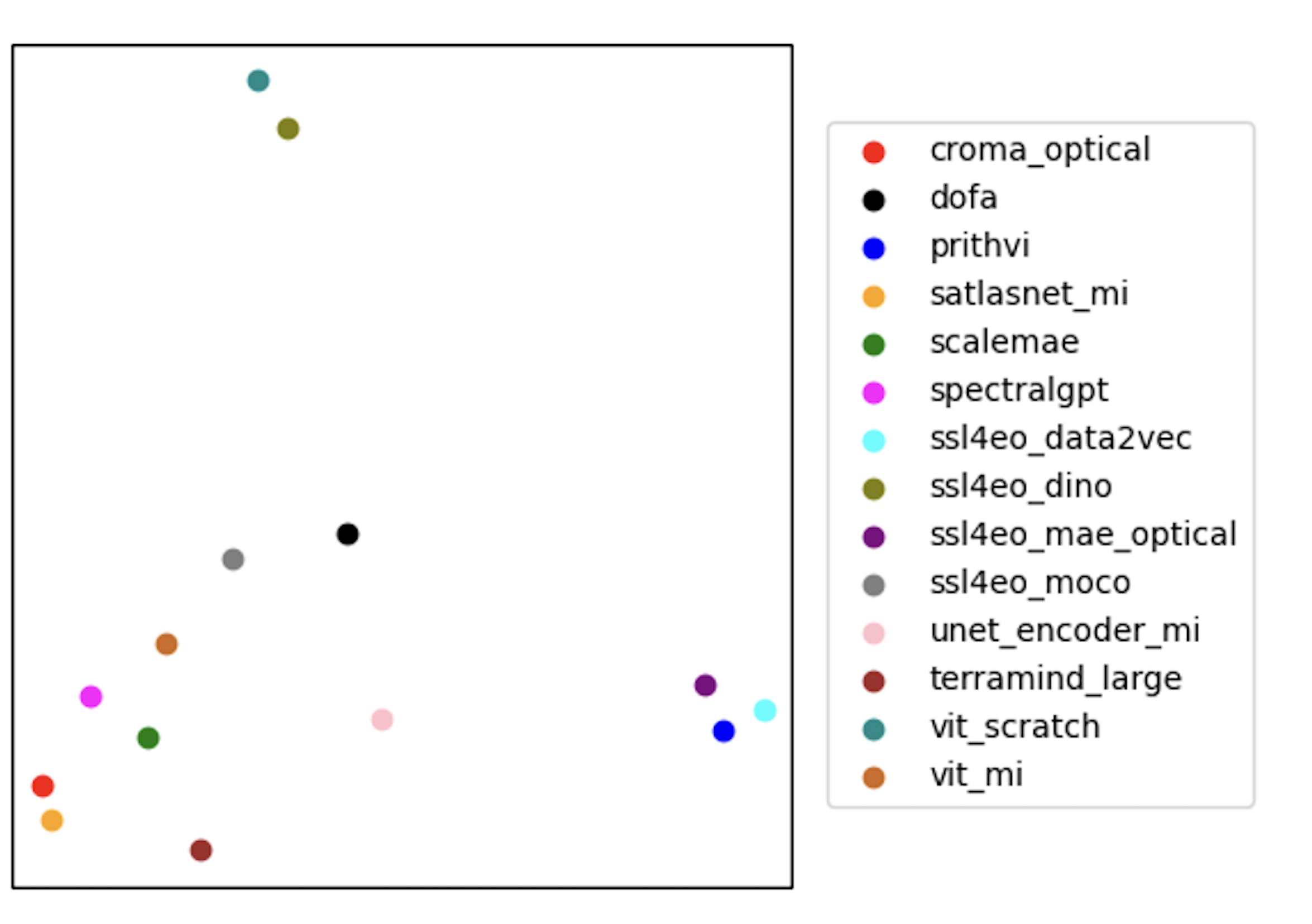
In the reduced-dimension single-point mapping in Figure 23, we can see that CROMA, DOFA, and Prithvi are all in distinct clusters, meaning that this measure of their representational structure shows strong distinctions. This gives us one point of information in our model selection and representation analysis journey, but should not be used as a comprehensive indicator on its own.

Distance matrix plot of collapsed embedding spaces for MTBS models

Distance matrix plot of collapsed embedding spaces for MTBS models
Figure 23. A depiction of collapsing the embedding spaces into single points to visualize and measure population-level representational differences for the MTBS dataset test case.


Figures 24 and 25 show different visualizations from pairwise comparisons of the p-value distributions of differences between the two representations of the same samples, as described above. Here, we can see that the representations are distinct. This is demonstrated by the number of samples with low p-values and by the p-value distribution plots in Figure 25, which show strong leftward shifts. In this case, no model’s class separation really stands out in the UMAP plots, and all models have distinct representations.

Scatterplots comparing pairwise representational similarity between models using p-values, MTBS data

Scatterplots comparing pairwise representational similarity between models using p-values, MTBS data
Figure 24. Scatterplots of the MTBS embedding projections being used to measure population-level representational shifts between pairs of models. Here, the sample set from the model being compared against is plotted, and the model we are measuring deviation from has its samples overlaid on top. The opacity has an inverse relationship to the p-value of a given sample. All values with a p-value close to or equal to 1 are colored white here and therefore do not show up. Comparison datasets are on the left of the arrow and reference datasets are on the right for each plot title.


Distribution plots of p-values for each pair of models, MTBS dataset

Distribution plots of p-values for each pair of models, MTBS dataset
Figure 25. The distribution of p-values under the null hypothesis for each ordered pair of models and the MTBS data. Comparison datasets are on the left of the arrow and reference datasets are on the right for each plot title.


The comparison of Prithvi and CROMA samples (center top and bottom) demonstrates a similar phenomenon as the ones described in the previous case. Again, when Prithvi embeddings are held as the reference set and CROMA as the comparison set (center top), we get a lessened measure of similarity. At the same time, we move closer to a full acceptance of the null hypothesis when the roles of the datasets are swapped. This is due to the difference in spread between each model’s samples in the collective embedding space. The rejection radius for CROMA is larger than for Prithvi, given the spread of a larger set of samples from CROMA. Thus, when we use CROMA as reference, more sample tests accept the null hypothesis. The difference is similar, but shifted towards hypothesis acceptance when looking at the plots for DOFA and Prithvi because a larger density of CROMA’s embeddings is farther away from that of Prithvi’s, when compared to DOFA’s. The case is very similar when comparing DOFA and CROMA. We can see these patterns show up in the density-scaled scatter plots in Figure 17 as well as the inverse-p-value scaled ones in Figure 19. Again, this is consistent with the varying qualities observed in Figures 16 & 17.

Variability and spread

Models produce distinct representations even when given the same input. This arises from differences in architecture, training data, and objectives, leading to varying interpretations that affect performance, generalizability, and trust in model outputs. This distinction is especially important when considering the encoder component, which is solely responsible for transforming raw input into that latent representation. Since the encoder defines what information is preserved, emphasized, or discarded, any differences in its learned mapping directly shape the structure and spread of the embedding space. For instance, two encoders may process the same image and yield representations that differ not just in detail, but in what aspects of the scene are even considered salient, such as texture vs. shape, global vs. local features, or background vs. foreground elements.

With that said, greater variability and spread in the projected embedding space, as in the case of the CROMA model, does not necessarily translate to improved utility. A model with a more diffuse spread may have greater capacity to separate subtle differences between input types, yet it may also be vulnerable to noise or irrelevant distinctions. This added burden can lead to increased complexity in downstream task design, reduced robustness, or even degraded performance if the embeddings fail to cluster relevantly similar inputs for the task at hand. In such cases, the downstream model must work harder to reimpose structure on a representation space that is less naturally organized, potentially offsetting the advantages of the encoder’s expressiveness.

These tools can be used not only to intercompare distinct encoders, but also to visualize what happens to a model’s representations when processes are changed. For instance, they can be used to examine representational differences in a single encoder before and after fine-tuning, or across two different pretraining dataset splits (Duderstadt et al., 2023).

Identifying embedding-level differences and large-scale representation gaps is crucial and can be quantitatively measured using these tools. These methodologies for rigorously inter-comparing representational capabilities are crucial for both better understanding encoder performance and further architecture development.

Section D: Example Fine Tuning

Background

Now that we’ve established some of the major concepts underpinning the foundation models, we can move forward with fine-tuning the models. Along with the 3 FMs highlighted above, we will train the 5 different decoders described in section A for a total of 15 model variations. For comparative studies of foundation models, compute becomes a key bottleneck—especially when aiming for systematic comparisons across model tasks or training regimes. For the sake of this demonstration, we limit each training run to a batch size of 8 for 16 epochs on a single T4 GPU with 15GB of VRAM, within Google Colab.

We target two fire-related tasks: segmenting burn scars in HLS scenes and multiclass segmentation of burn intensity. Both are HLS-derived benchmarks, an input source that provides harmonized surface reflectance from three satellite missions (Landsat-8, Landsat-9, and Sentinel-2) and, in doing so, provides a relatively level testbed for models trained on either. Nevertheless, it’s important to acknowledge the nature of the benchmark datasets used. While they have been carefully curated to support robust model evaluation, it may not fully reflect the diversity or complexity of real-world fire scenarios with potentially drastically different landscape dynamics, data availability, and task scope. The dataset is limited in geographic scope, vegetation types, and imaging conditions, which means performance metrics obtained here may not generalize well to all fire contexts, such as risk mapping. As such, results from this benchmark should be interpreted with consideration of these constraints.

HLS BURN SCARS Training Commands

Show code
%%time


#Move up to the main directory of the pangaea lib
%cd /content

%env WANDB_MODE=offline

# DOFA

!torchrun pangaea-bench/pangaea/run.py \
    --config-name=train \
    work_dir=checkpoints \
    dataset=hlsburnscars \
    encoder=dofa\
    decoder=seg_muster\
    preprocessing=seg_irregular_images\
    criterion=cross_entropy \
    task=segmentation \
    use_wandb=true \
    task.trainer.n_epochs=16 \
    task.trainer.log_interval=1 \
    task.trainer.ckpt_interval=16 \
    encoder.encoder_weights=pretrained_models/DOFA_ViT_base_e100.pth

!torchrun pangaea-bench/pangaea/run.py \
    --config-name=train \
    work_dir=checkpoints \
    dataset=hlsburnscars \
    encoder=dofa\
    decoder=seg_fcn\
    preprocessing=seg_irregular_images\
    criterion=cross_entropy \
    task=segmentation \
    use_wandb=true \
    task.trainer.n_epochs=16 \
    task.trainer.log_interval=1 \
    task.trainer.ckpt_interval=16 \
    encoder.encoder_weights=pretrained_models/DOFA_ViT_base_e100.pth

!torchrun pangaea-bench/pangaea/run.py \
    --config-name=train \
    work_dir=checkpoints \
    dataset=hlsburnscars \
    encoder=dofa\
    decoder=seg_linear\
    preprocessing=seg_irregular_images\
    criterion=cross_entropy \
    task=segmentation \
    use_wandb=true \
    task.trainer.n_epochs=16 \
    task.trainer.log_interval=1 \
    task.trainer.ckpt_interval=16 \
    encoder.encoder_weights=pretrained_models/DOFA_ViT_base_e100.pth

!torchrun pangaea-bench/pangaea/run.py \
    --config-name=train \
    work_dir=checkpoints \
    dataset=hlsburnscars \
    encoder=dofa\
    decoder=seg_segformer\
    preprocessing=seg_irregular_images \
    criterion=cross_entropy \
    task=segmentation \
    use_wandb=true \
    task.trainer.n_epochs=16 \
    task.trainer.log_interval=1 \
    task.trainer.ckpt_interval=16 \
    encoder.encoder_weights=pretrained_models/DOFA_ViT_base_e100.pth

!torchrun pangaea-bench/pangaea/run.py \
    --config-name=train \
    work_dir=checkpoints \
    dataset=hlsburnscars \
    encoder=dofa\
    decoder=seg_upernet\
    preprocessing=seg_irregular_images \
    criterion=cross_entropy \
    task=segmentation \
    use_wandb=true \
    task.trainer.n_epochs=16 \
    task.trainer.log_interval=1 \
    task.trainer.ckpt_interval=16 \
    encoder.encoder_weights=pretrained_models/DOFA_ViT_base_e100.pth

## PRITHVI

!torchrun pangaea-bench/pangaea/run.py \
    --config-name=train \
    work_dir=checkpoints \
    dataset=hlsburnscars \
    encoder=prithvi \
    decoder=seg_muster\
    preprocessing=seg_irregular_images \
    criterion=cross_entropy \
    task=segmentation \
    use_wandb=true \
    task.trainer.n_epochs=16 \
    task.trainer.log_interval=1 \
    task.trainer.ckpt_interval=16 \
    encoder.encoder_weights=pretrained_models/Prithvi_EO_V1_100M.pt

!torchrun pangaea-bench/pangaea/run.py \
    --config-name=train \
    work_dir=checkpoints \
    dataset=hlsburnscars \
    encoder=prithvi \
    decoder=seg_fcn\
    preprocessing=seg_irregular_images \
    criterion=cross_entropy \
    task=segmentation \
    use_wandb=true \
    task.trainer.n_epochs=16 \
    task.trainer.log_interval=1 \
    task.trainer.ckpt_interval=16 \
    encoder.encoder_weights=pretrained_models/Prithvi_EO_V1_100M.pt

!torchrun pangaea-bench/pangaea/run.py \
    --config-name=train \
    work_dir=checkpoints \
    dataset=hlsburnscars \
    encoder=prithvi \
    decoder=seg_linear\
    preprocessing=seg_irregular_images \
    criterion=cross_entropy \
    task=segmentation \
    use_wandb=true \
    task.trainer.n_epochs=16 \
    task.trainer.log_interval=1 \
    task.trainer.ckpt_interval=16 \
    encoder.encoder_weights=pretrained_models/Prithvi_EO_V1_100M.pt

!torchrun pangaea-bench/pangaea/run.py \
    --config-name=train \
    work_dir=checkpoints \
    dataset=hlsburnscars \
    encoder=prithvi\
    decoder=seg_segformer\
    preprocessing=seg_irregular_images \
    criterion=cross_entropy \
    task=segmentation \
    use_wandb=true \
    task.trainer.n_epochs=16 \
    task.trainer.log_interval=1 \
    task.trainer.ckpt_interval=16 \
    encoder.encoder_weights=pretrained_models/Prithvi_EO_V1_100M.pt

!torchrun pangaea-bench/pangaea/run.py \
    --config-name=train \
    work_dir=checkpoints \
    dataset=mtbs \
    encoder=prithvi \
    decoder=seg_upernet\
    preprocessing=seg_irregular_images \
    criterion=cross_entropy \
    task=segmentation \
    use_wandb=true \
    task.trainer.n_epochs=16 \
    task.trainer.log_interval=1 \
    task.trainer.ckpt_interval=16 \
    encoder.encoder_weights=pretrained_models/Prithvi_EO_V1_100M.pt

## CROMA

!torchrun pangaea-bench/pangaea/run.py \
    --config-name=train \
    work_dir=checkpoints \
    dataset=hlsburnscars \
    encoder=croma_optical\
    decoder=seg_muster\
    preprocessing=seg_irregular_images \
    criterion=cross_entropy \
    task=segmentation \
    use_wandb=true \
    task.trainer.n_epochs=16 \
    task.trainer.log_interval=1 \
    task.trainer.ckpt_interval=16 \
    encoder.encoder_weights=pretrained_models/CROMA_large.pt

!torchrun pangaea-bench/pangaea/run.py \
    --config-name=train \
    work_dir=checkpoints \
    dataset=hlsburnscars \
    encoder=croma_optical\
    decoder=seg_fcn\
    preprocessing=seg_irregular_images \
    criterion=cross_entropy \
    task=segmentation \
    use_wandb=true \
    task.trainer.n_epochs=16 \
    task.trainer.log_interval=1 \
    task.trainer.ckpt_interval=16 \
    encoder.encoder_weights=pretrained_models/CROMA_large.pt

!torchrun pangaea-bench/pangaea/run.py \
    --config-name=train \
    work_dir=checkpoints \
    dataset=hlsburnscars \
    encoder=croma_optical\
    decoder=seg_linear\
    preprocessing=seg_irregular_images \
    criterion=cross_entropy \
    task=segmentation \
    use_wandb=true \
    task.trainer.n_epochs=16 \
    task.trainer.log_interval=1 \
    task.trainer.ckpt_interval=16 \
    encoder.encoder_weights=pretrained_models/CROMA_large.pt

!torchrun pangaea-bench/pangaea/run.py \
    --config-name=train \
    work_dir=checkpoints \
    dataset=hlsburnscars \
    encoder=croma_optical\
    decoder=seg_segformer\
    preprocessing=seg_irregular_images \
    criterion=cross_entropy \
    task=segmentation \
    use_wandb=true \
    task.trainer.n_epochs=16 \
    task.trainer.log_interval=1 \
    task.trainer.ckpt_interval=16 \
    encoder.encoder_weights=pretrained_models/CROMA_large.pt

!torchrun pangaea-bench/pangaea/run.py \
    --config-name=train \
    work_dir=checkpoints \
    dataset=hlsburnscars \
    encoder=croma_optical\
    decoder=seg_upernet\
    preprocessing=seg_irregular_images \
    criterion=cross_entropy \
    task=segmentation \
    use_wandb=true \
    task.trainer.n_epochs=16 \
    task.trainer.log_interval=1 \
    task.trainer.ckpt_interval=16 \
    encoder.encoder_weights=pretrained_models/CROMA_large.pt

HLS BURN SCARS Results

Some things to consider:

Below, Figure 26 depicts the results from running the above commands aggregated into relatively simple charts. Keep in mind that we only train for 16 epochs for a simple demonstration. This is a very small amount of time for a deep learning model. There is a reasonable chance that these metrics will change given enough training time, a different loss function, or a different set of hyperparameters. The framework allows for some level of configuration. On your own, try setting new configurations (see ./pangaea-bench/configs for details).

Training Graphs

Despite a limited training window, we see a fairly distinct training curve, which suggests the models have learned some useful features. Whether this is due to the pretraining or the simple nature of the task is still an open question. A straightforward test for that is to train using a randomly initialized encoder by adjusting the last configuration in each training command to null. In addition, there is a clear loss difference between the models, with DOFA generally having a higher cross-entropy loss.

Line chart of training loss per step for all model variations

Line chart of training loss per step for all model variations
Figure 26: Training loss per step for all model variations. Each model was optimized using cross-entropy loss.


Decoder Choice

The test metrics for the checkpoint saved at the final epoch, shown in Figure 29, tell a slightly different story. Overall, the CROMA combinations appear to be the most effective in terms of overall performance metrics (F1 and IoU). The PRITHVI encoder consistently shows good performance across different decoders, with the Linear Probe surprisingly being the top performer in this group. The DOFA Linear Probe combination stands out as an outlier with extremely low performance for burn scar detection. The lower performance of the probe into DOFA suggests its internal representation may not be appropriate for this task, and the decoder might be doing the bulk of the heavy lifting in the other runs, which aligns with our evaluation of the encoder analysis in the above sections. More experimentation is required to confirm this. It’s worth noting that even with the same encoder, varying the decoder has a visible effect on performance that is comparable in magnitude to the differences between encoders.

Bar chart of test metrics for each encoder-decoder combination

Bar chart of test metrics for each encoder-decoder combination
Figure 27: Test metrics per encoder-decoder variation

Per Class Metrics

Looking at per-class metrics in Figure 28 gives a bit more insight into what’s happening. Aside from the DOFA-linear-probe outlier, the differences from model to model are realistically negligible, although further statistical testing would be recommended to confirm this. However, when we look at per-class metrics, we see a more noticeable difference between each model’s ability to segment the positive class. This suggests a class imbalance issue. While this may accurately reflect the task, it needs to be taken into account when designing a benchmark dataset and evaluation framework.

Bar chart of per-class performance metrics for each model

Bar chart of per-class performance metrics for each model
Figure 28: Per class metrics


Run Times and Compute Costs

Based on the above metrics alone, CROMA seems to be a top performer; nevertheless, we must consider one more aspect: compute. In Figure 29, we see that CROMA consumed up to ~3 times the memory and up to ~9 times the training time as some of the other models for the same number of epochs. This is consistent with the FLOP calculations found in Table 1. This is likely due to the large number of dimensions in the released CROMA model compared to its peers (1024 as opposed to more common 768). In other words, for the same resources, DOFA combined with an even larger decoder trained for 128 epochs instead of 16 may very well outperform the CROMA models. In the same vein, Prithvi consumed a comparable amount of memory to CROMA but is far simpler to implement and fine-tunes several times faster. Theoretically, these models are modular and can be compared at a variety of sizes for each model. However, most models are released with pretrained versions only at a single size, so comparisons must be taken as-is.

Bar chart of GPU memory usage per encoder-decoder combination

Bar chart of GPU memory usage per encoder-decoder combination

Bar chart of training run time in seconds for each model

Bar chart of training run time in seconds for each model
Figure 29: (Top) GPU VRAM usage per encoder-decoder combination. (Bottom) Run time in seconds to reach 16 epochs.


Output Masks

We have all these metrics, and they all tell a similar story. The first thing you should notice from Figure 30 is that the annotation is not perfect. So the metrics above should be interpreted carefully. For example, the Prithvi masks from all decoders look vastly different while the metrics say otherwise. When the benchmark dataset was created, chip labels with multiple annotations in proximity were likely left unfiltered. This does offer an opportunity to see how a model behaves in such situations, which are unfortunately all too common. Interestingly, whether or not the model captures the false negatives depends mostly on the decoder. In addition, artifacts in the images arise from the structure of the decoder itself rather than anything meaningful in the image.

Grid of predicted segmentation masks from all model and decoder combinations

Grid of predicted segmentation masks from all model and decoder combinations

Original ground truth annotation mask for the HLS burn scar sample Source satellite image corresponding to the HLS burn scar sample

Figure 30: (Top) Grid table of mask outputs of all models with all decoders. (Bottom Left) Original annotation. (Bottom Right) Source Image

Multimodality / Multisensor Models Scale

You may have noticed that, despite being a small decoder, the linear probe into PRITHVI had comparable performance to the larger models in this given task. While this may be attributed to the limited training time or architectural design choices, the more likely reason is that PRITHVI 1.0 was trained exclusively on HLS scenes. Foundation Models, like all machine learning models, are shaped by their source data, and making them truly generalizable is an ongoing problem. Likewise, spatiotemporal patterns are diverse in both downstream tasks and sensor data. Ultimately, when selecting a base model, one of the first things to consider before benchmarking metrics is how well the pretraining dataset aligns with your given task.

MTBS Training Commands

While it is an excellent example for learning to fine-tune due to its small size and simplistic design, it may be difficult to differentiate model utility with the HLS burn scar dataset. Next, we’ll examine the dataset on which we performed the encoder analysis by running the same commands as the previous section, with the dataset configuration set to mtbs. Luckily for us, we’ve also implemented the dataloader and configurations found in ./pangaea-bench/pangaea and ./pangaea-bench/configs, respectively. Since this is a much larger dataset (5 times in fact), these runs may take up to two hours to run rather than a few minutes.

Show code
%%time

#Move up to the main directory of the pangaea lib
%cd /content

%env WANDB_MODE=offline

# CROMA

!torchrun pangaea-bench/pangaea/run.py \
    --config-name=train \
    work_dir=checkpoints \
    dataset=mtbs \
    encoder=croma_optical\
    decoder=seg_muster\
    preprocessing=seg_irregular_images \
    criterion=cross_entropy \
    task=segmentation \
    use_wandb=true \
    task.trainer.n_epochs=16 \
    task.trainer.log_interval=1 \
    task.trainer.ckpt_interval=16 \
    encoder.encoder_weights=pretrained_models/CROMA_large.pt

!torchrun pangaea-bench/pangaea/run.py \
    --config-name=train \
    work_dir=checkpoints \
    dataset=mtbs \
    encoder=croma_optical\
    decoder=seg_fcn\
    preprocessing=seg_irregular_images \
    criterion=cross_entropy \
    task=segmentation \
    use_wandb=true \
    task.trainer.n_epochs=16 \
    task.trainer.log_interval=1 \
    task.trainer.ckpt_interval=16 \
    encoder.encoder_weights=pretrained_models/CROMA_large.pt

!torchrun pangaea-bench/pangaea/run.py \
    --config-name=train \
    work_dir=checkpoints \
    dataset=mtbs \
    encoder=croma_optical\
    decoder=seg_linear\
    preprocessing=seg_irregular_images \
    criterion=cross_entropy \
    task=segmentation \
    use_wandb=true \
    task.trainer.n_epochs=16 \
    task.trainer.log_interval=1 \
    task.trainer.ckpt_interval=16 \
    encoder.encoder_weights=pretrained_models/CROMA_large.pt

!torchrun pangaea-bench/pangaea/run.py \
    --config-name=train \
    work_dir=checkpoints \
    dataset=mtbs \
    encoder=croma_optical\
    decoder=seg_segformer\
    preprocessing=seg_irregular_images \
    criterion=cross_entropy \
    task=segmentation \
    use_wandb=true \
    task.trainer.n_epochs=16 \
    task.trainer.log_interval=1 \
    task.trainer.ckpt_interval=16 \
    encoder.encoder_weights=pretrained_models/CROMA_large.pt

!torchrun pangaea-bench/pangaea/run.py \
    --config-name=train \
    work_dir=checkpoints \
    dataset=mtbs \
    encoder=croma_optical\
    decoder=seg_upernet\
    preprocessing=seg_irregular_images \
    criterion=cross_entropy \
    task=segmentation \
    use_wandb=true \
    task.trainer.n_epochs=16 \
    task.trainer.log_interval=1 \
    task.trainer.ckpt_interval=16 \
    encoder.encoder_weights=pretrained_models/CROMA_large.pt

## PRITHVI

!torchrun pangaea-bench/pangaea/run.py \
    --config-name=train \
    work_dir=checkpoints \
    dataset=mtbs \
    encoder=prithvi\
    decoder=seg_muster\
    preprocessing=seg_irregular_images \
    criterion=cross_entropy \
    task=segmentation \
    use_wandb=true \
    task.trainer.n_epochs=16 \
    task.trainer.log_interval=1 \
    task.trainer.ckpt_interval=16 \
    encoder.encoder_weights=pretrained_models/Prithvi_EO_V1_100M.pt

!torchrun pangaea-bench/pangaea/run.py \
    --config-name=train \
    work_dir=checkpoints \
    dataset=mtbs \
    encoder=prithvi\
    decoder=seg_fcn\
    preprocessing=seg_irregular_images \
    criterion=cross_entropy \
    task=segmentation \
    use_wandb=true \
    task.trainer.n_epochs=16 \
    task.trainer.log_interval=1 \
    task.trainer.ckpt_interval=16 \
    encoder.encoder_weights=pretrained_models/Prithvi_EO_V1_100M.pt

!torchrun pangaea-bench/pangaea/run.py \
    --config-name=train \
    work_dir=checkpoints \
    dataset=mtbs \
    encoder=prithvi\
    decoder=seg_linear\
    preprocessing=seg_irregular_images \
    criterion=cross_entropy \
    task=segmentation \
    use_wandb=true \
    task.trainer.n_epochs=16 \
    task.trainer.log_interval=1 \
    task.trainer.ckpt_interval=16 \
    encoder.encoder_weights=pretrained_models/Prithvi_EO_V1_100M.pt

!torchrun pangaea-bench/pangaea/run.py \
    --config-name=train \
    work_dir=checkpoints \
    dataset=mtbs \
    encoder=prithvi\
    decoder=seg_segformer\
    preprocessing=seg_irregular_images \
    criterion=cross_entropy \
    task=segmentation \
    use_wandb=true \
    task.trainer.n_epochs=16 \
    task.trainer.log_interval=1 \
    task.trainer.ckpt_interval=16 \
    encoder.encoder_weights=pretrained_models/Prithvi_EO_V1_100M.pt

!torchrun pangaea-bench/pangaea/run.py \
    --config-name=train \
    work_dir=checkpoints \
    dataset=mtbs \
    encoder=prithvi\
    decoder=seg_upernet\
    preprocessing=seg_irregular_images \
    criterion=cross_entropy \
    task=segmentation \
    use_wandb=true \
    task.trainer.n_epochs=16 \
    task.trainer.log_interval=1 \
    task.trainer.ckpt_interval=16 \
    encoder.encoder_weights=pretrained_models/Prithvi_EO_V1_100M.pt

## DOFA

!torchrun pangaea-bench/pangaea/run.py \
    --config-name=train \
    work_dir=checkpoints \
    dataset=mtbs \
    encoder=dofa \
    decoder=seg_muster\
    preprocessing=seg_irregular_images \
    criterion=cross_entropy \
    task=segmentation \
    use_wandb=true \
    task.trainer.n_epochs=16 \
    task.trainer.log_interval=1 \
    task.trainer.ckpt_interval=16 \
    encoder.encoder_weights=pretrained_models/DOFA_ViT_base_e100.pth

!torchrun pangaea-bench/pangaea/run.py \
    --config-name=train \
    work_dir=checkpoints \
    dataset=mtbs \
    encoder=dofa\
    decoder=seg_fcn\
    preprocessing=seg_irregular_images \
    criterion=cross_entropy \
    task=segmentation \
    use_wandb=true \
    task.trainer.n_epochs=16 \
    task.trainer.log_interval=1 \
    task.trainer.ckpt_interval=16 \
    encoder.encoder_weights=pretrained_models/DOFA_ViT_base_e100.pth

!torchrun pangaea-bench/pangaea/run.py \
    --config-name=train \
    work_dir=checkpoints \
    dataset=mtbs \
    encoder=dofa\
    decoder=seg_linear\
    preprocessing=seg_irregular_images \
    criterion=cross_entropy \
    task=segmentation \
    use_wandb=true \
    task.trainer.n_epochs=16 \
    task.trainer.log_interval=1 \
    task.trainer.ckpt_interval=16 \
    encoder.encoder_weights=pretrained_models/DOFA_ViT_base_e100.pth

!torchrun pangaea-bench/pangaea/run.py \
    --config-name=train \
    work_dir=checkpoints \
    dataset=mtbs \
    encoder=dofa\
    decoder=seg_segformer\
    preprocessing=seg_irregular_images \
    criterion=cross_entropy \
    task=segmentation \
    use_wandb=true \
    task.trainer.n_epochs=16 \
    task.trainer.log_interval=1 \
    task.trainer.ckpt_interval=16 \
    encoder.encoder_weights=pretrained_models/DOFA_ViT_base_e100.pth

!torchrun pangaea-bench/pangaea/run.py \
    --config-name=train \
    work_dir=checkpoints \
    dataset=mtbs \
    encoder=dofa\
    decoder=seg_upernet\
    preprocessing=seg_irregular_images \
    criterion=cross_entropy \
    task=segmentation \
    use_wandb=true \
    task.trainer.n_epochs=16 \
    task.trainer.log_interval=1 \
    task.trainer.ckpt_interval=16 \
    encoder.encoder_weights=pretrained_models/DOFA_ViT_base_e100.pth

MTBS Results

Overall Metrics

Unlike the previous task, Figure 31 shows markedly poorer results. Using the typical hyperparameter settings a practitioner would apply in their first pass (i.e., cross-entropy loss, moderate learning rate, etc.), we find that this is insufficient to produce meaningful results. Understandably, the burn intensity dataset has a greater number of classes, an additional temporal reasoning component, and regional differences that are not depicted here. Burn severity labels themselves are highly contextual, with evaluation for each fire and each region specific to those contexts, creating a very difficult challenge for all of our models. These results are also consistent with the embedding analysis in Figure 17, where we see limited separation between classes. Clever fine-tuning techniques may be able to compensate for these shortcomings; however, they could negate any pretraining benefits and, worse still, may not achieve comparable results to an end-to-end trained network.

Bar chart of best test metrics per encoder and decoder combination, MTBS

Bar chart of best test metrics per encoder and decoder combination, MTBS
Figure 31: Best metrics per best decoder with each encoder.

Interpretation

Change detection/attribution is a difficult topic, as even the veterans of the remote sensing world will tell you. It is often multivariate and involves very subtle landscape dynamics which are not clear to the human eye without aid. For example, Figure 32 shows a sample pulled from the MTBS dataset. These are scenes from the Boulder Lake, WA Fire in August 2022. Between the second and third image, it is clear where the fire had occurred (vegetation turned to bare soil) despite the smoke and other artifacts in the third image. Given our results from the first fine-tuning workflow, detecting this would be easy for all models. Yet when we extend the problem to intensity, the model must additionally reason what vegetation was present before the fire, what vegetation died, and also what vegetation experienced a low enough fire temperature to survive and regrow the following year, all while contending with the strong noisy signals ever present in all images and the variations between them. An extremely complex task.

Landsat image of Boulder Lake, Washington one year before the 2022 fire Landsat image of Boulder Lake, Washington two months after the 2022 fire Landsat image of Boulder Lake, Washington one year after the 2022 fire Landsat image of Boulder Lake, Washington two years after the 2022 fire

(a)

Landsat image of Boulder Lake, Washington two years post-fire with burn severity labels overlaid

Landsat image of Boulder Lake, Washington two years post-fire with burn severity labels overlaid
(b)
Figure 32: (a) Landsat imagery from the Boulder Lake, WA fire in August 2022. From left to right: 1 year pre-fire, 2 months post-fire, 1 year post-fire, 2 years post-fire. (b) 2-year post-fire with class labels overlaid.

A Well-Defined Problem

Benchmarks such as ImageNet for vision tasks or GLUE for language tasks have helped standardize comparisons, but emerging domains may lack such comprehensive baselines. In such cases, creating task-specific benchmarks becomes more necessary, especially as these “Foundation Models” become more prominent. Like all standardized evaluations, benchmarks can often promote excessive metric fixation. Even so, these metrics are necessary when comparing across models and must be done under the same conditions: using the same dataset splits, preprocessing steps, and evaluation protocols. Differences in any of these factors can distort the interpretation of results. For that reason, we see testing in multiple controlled conditions as an essential step for a robust evaluation. In our simplified example above, we vary the decoder attached to each frozen pretrained encoder, as the quality of the internal representation is only as good as how easily we can extract from it. Model complexity, training time, and inference speed are also crucial metrics to consider, especially in deployment scenarios where computational resources or latency requirements are constrained. Lastly, assessing representation quality is important for determining whether the architecture, pretraining task, or both contribute to the model’s overall performance. While this process may seem overwhelming and extensive at first, we hope that you can use these guidelines to develop a strong practice of intensive validation and model evaluation, which will, in turn, provide larger benefits to your work and area of interest. This level of care and rigor must go into the evaluation of representation and performance to ensure that these function approximators are actually aiding in scientific discovery and other downstream tasks, and not just creating additional new webs of questions to disentangle. This should not be seen as an unpassable barrier, but a challenge and a standard that will allow us all to work together to improve capabilities in scientific understanding and geospatial intelligence.

References

  1. Alain, G., & Bengio, Y. (2016, October 5). Understanding intermediate layers using linear classifier probes. arXiv.org. https://arxiv.org/abs/1610.01644

  2. Bommasani, R., Hudson, D. A., Adeli, E., Altman, R., Arora, S., von Arx, S., Bernstein, M. S., Bohg, J., Bosselut, A., Brunskill, E., Brynjolfsson, E., Buch, S., Card, D., Castellon, R., Chatterji, N., Chen, A., Creel, K., Davis, J. Q., Demszky, D., … Liang, P. (2021). On the Opportunities and Risks of Foundation Models (Version 3). arXiv. https://doi.org/10.48550/ARXIV.2108.07258

  3. Caron, M., Touvron, H., Misra, I., Jégou, H., Mairal, J., Bojanowski, P., & Joulin, A. (2021, April 29). Emerging Properties in Self-Supervised Vision Transformers. arXiv.org. https://arxiv.org/abs/2104.14294

  4. Chen, T., Kornblith, S., Norouzi, M., & Hinton, G. (2020, February 13). A simple framework for contrastive learning of visual representations. arXiv.org. https://arxiv.org/abs/2002.05709

  5. Cocke, A. E., Fulé, P. Z., & Crouse, J. E. (2005). Comparison of burn severity assessments using Differenced Normalized Burn Ratio and ground data. International Journal of Wildland Fire, 14(2), 189–198. https://doi.org/10.1071/wf04010

  6. DeMilt, R. P., LaHaye, N., & Tenneson, K. (2026). The View From Space: Navigating Instrumentation Differences with EOFMs. Machine Learning and the Physical Sciences Workshop @ NeurIPS 2025. Machine Learning and the Physical Sciences Workshop @ NeurIPS 2025. https://openreview.net/forum?id=qqwMYRjgbQ

  7. Duderstadt, B., Helm, H. S., & Priebe, C. E. (2023, May 9). Comparing Foundation Models using Data Kernels. arXiv.org. https://arxiv.org/abs/2305.05126

  8. Grill, J., Strub, F., Altché, F., Tallec, C., Richemond, P. H., Buchatskaya, E., Doersch, C., Pires, B. A., Guo, Z. D., Azar, M. G., Piot, B., Kavukcuoglu, K., Munos, R., & Valko, M. (2020, June 13). Bootstrap your own latent: A new approach to self-supervised Learning. arXiv.org. https://arxiv.org/abs/2006.07733

  9. Han K, Wang Y, Chen H, Chen X, Guo J, Liu Z, Tang Y, Xiao A, Xu C, Xu Y, Yang Z, Zhang Y, Tao D. A Survey on Vision Transformer. IEEE Trans Pattern Anal Mach Intell. 2023 Jan;45(1):87-110. doi: 10.1109/TPAMI.2022.3152247. Epub 2022 Dec 5. PMID: 35180075.

  10. He, K., Fan, H., Wu, Y., Xie, S. and Girshick, R., “Momentum Contrast for Unsupervised Visual Representation Learning,” 2020 IEEE/CVF Conference on Computer Vision and Pattern Recognition (CVPR), Seattle, WA, USA, 2020, pp. 9726-9735, doi: 10.1109/CVPR42600.2020.00975.

  11. He, K., Chen, X., Xie, S., Li, Y., Dollár, P. and Girshick, R., “Masked Autoencoders Are Scalable Vision Learners,” 2022 IEEE/CVF Conference on Computer Vision and Pattern Recognition (CVPR), New Orleans, LA, USA, 2022, pp. 15979-15988, doi: 10.1109/CVPR52688.2022.01553.

  12. Jakubik, J., Roy, S., Phillips, C. E., Fraccaro, P., Godwin, D., Zadrozny, B., Szwarcman, D., Gomes, C., Nyirjesy, G., Edwards, B., Kimura, D., Simumba, N., Chu, L., Mukkavilli, S. K., Lambhate, D., Das, K., Bangalore, R., Oliveira, D., Muszynski, M., . . . Ramachandran, R. (2023b, October 28). Foundation Models for Generalist Geospatial Artificial Intelligence. arXiv.org. https://arxiv.org/abs/2310.18660

  13. Kolesnikov, A., Dosovitskiy, A., Weissenborn, D., Heigold, G., Uszkoreit, J., Beyer, L., Minderer, M., Dehghani, M., Houlsby, N., Gelly, S., Unterthiner, T., & Zhai, X. (2021). An Image is Worth 16x16 Words: Transformers for Image Recognition at Scale.

  14. LaHaye, N., Garay, M. J., Bue, B. D., El-Askary, H., & Linstead, E. (2021). A Quantitative Validation of Multi-Modal Image Fusion and Segmentation for Object Detection and Tracking. Remote Sensing, 13(12), 2364. https://doi.org/10.3390/rs13122364

  15. Long, J., Shelhamer, E., & Darrell, T. (2014, November 14). Fully convolutional networks for semantic segmentation. arXiv.org. https://arxiv.org/abs/1411.4038

  16. Marsocci, V., Jia, Y., Bellier, G. L., Kerekes, D., Zeng, L., Hafner, S., Gerard, S., Brune, E., Yadav, R., Shibli, A., Fang, H., Ban, Y., Vergauwen, M., Audebert, N., & Nascetti, A. (2024, December 5). PANGAEA: a global and inclusive benchmark for Geospatial foundation models. arXiv.org. https://arxiv.org/abs/2412.04204

  17. Martin, Charles H., Mahoney, Michael W.; Implicit Self-Regularization in Deep Neural Networks: Evidence from Random Matrix Theory and Implications for Learning. JMLR 22(165):1−73, 2021

  18. Martin, Charles H., Peng, Tongsu (Serena) & Mahoney, Michael W. ; Predicting trends in the quality of state-of-the-art neural networks without access to training or testing data. Nature Communications 12(4122), 2021

  19. McInnes, Leland, Healy, John, & Melville, James. “UMAP: Uniform Manifold Approximation and Projection for Dimension Reduction.” arXiv preprint arXiv:1802.03426, 2020

  20. Parajuli, P., Shinde, R., Gurung, I., Maskey, M., & Ramachandran, R. (2024). Curating AI-Ready datasets for equity and Environmental Justice: A Data-Centric AI case study. IGARSS 2022 - 2022 IEEE International Geoscience and Remote Sensing Symposium, 483–487. https://doi.org/10.1109/igarss53475.2024.10641786

  21. Patterson, D., Gonzalez, J., Le, Q., Liang, C., Munguia, L., Rothchild, D., So, D., Texier, M., & Dean, J. (2021, April 21). Carbon emissions and large neural network training. arXiv.org. https://arxiv.org/abs/2104.10350

  22. Phillips, Christopher and Roy, Sujit and Ankur, Kumar and Ramachandran, Rahul. (2023, August). HLS Foundation Burnscars Dataset. https://huggingface.co/ibm-nasa-geospatial/hls_burn_scars

  23. Roy, D. P., Boschetti, L., & Trigg, S. N. (2006). Remote Sensing of Fire Severity: Assessing the Performance of the Normalized Burn Ratio. IEEE Geoscience and Remote Sensing Letters, 3(1), 112-116. https://doi.org/10.1109/lgrs.2005.858485

  24. Strubell, E., Ganesh, A., & McCallum, A. (2019, June 5). Energy and policy considerations for deep learning in NLP. arXiv.org. https://arxiv.org/abs/1906.02243

  25. Szwarcman, D., Roy, S., Fraccaro, P., Gíslason, O.E., Blumenstiel, B., Ghosal, R., De Oliveira, P.H., de Sousa Almeida, J.L., Sedona, R., Kang, Y. and Chakraborty, S., 2025. Prithvi-eo-2.0: A versatile multi-temporal foundation model for earth observation applications. IEEE Transactions on Geoscience and Remote Sensing.

  26. Vaswani, A., Shazeer, N., Parmar, N., Uszkoreit, J., Jones, L., Gomez, A. N., Kaiser, L., & Polosukhin, I. (2017). Attention Is All You Need (Version 7). arXiv. https://doi.org/10.48550/ARXIV.1706.03762

  27. Xiao, T., Liu, Y., Zhou, B., Jiang, Y., & Sun, J. (2018, July 26). Unified perceptual parsing for scene understanding. arXiv.org. https://arxiv.org/abs/1807.10221

  28. Xie, E., Wang, W., Yu, Z., Anandkumar, A., Alvarez, J. M., & Luo, P. (2021, May 31). SegFormer: Simple and Efficient Design for Semantic Segmentation with Transformers. arXiv.org. https://arxiv.org/abs/2105.15203

  29. Xiong, Z., Wang, Y., Zhang, F., Stewart, A. J., Hanna, J., Borth, D., Papoutsis, I., Saux, B. L., Camps-Valls, G., & Zhu, X. X. (2024, March 22). Neural Plasticity-Inspired multimodal foundation model for earth observation. arXiv.org. https://arxiv.org/abs/2403.15356

  30. Xu, J., Shi, W., Gao, P., Wang, Z., & Li, Q. (2022, November 25). MUSTER: a multi-scale transformer-based decoder for semantic segmentation. arXiv.org. https://arxiv.org/abs/2211.13928v2